Day 2 - Processing scRNAseq reads generated from Nextflow pipeline
Recap from Day 1
- Yesterday we covered:
- How to use Unix.
- How to get onto HAWK.
- How to fetch the Github repository and download the resources.
- How to execute the scrnaseq nextflow pipeline on Hawk.
Outputs from the nextflow pipeline
- The output from the nextflow execution run is stored under
results/cellranger_count_1k_mouse_kidney_CNIK_3pv3 - Login to your Hawk account and access the folder:
cd /scratch/c.123456/scrnaseq-course/scrnaseq/results

cd cellranger_count_1k_mouse_kidney_CNIK_3pv3
Downloading data for analysis in Seurat (for analysis on RStudio on local system)
- You can skip this step if you are working on RStudio Server.
- Once the counts are generated using nextflow pipeline, download the data onto your personal computer.
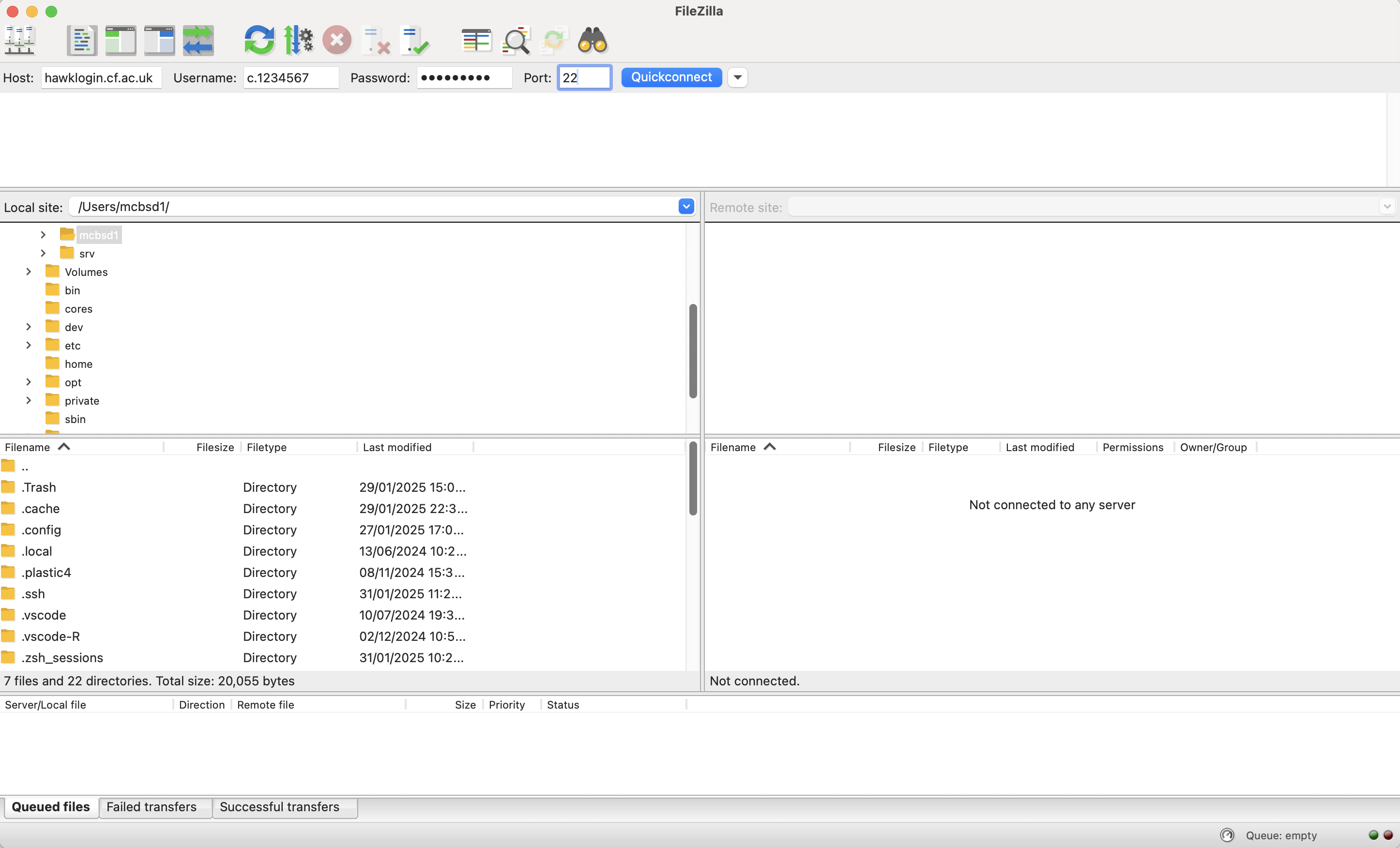
- For this, you will need to use Filezilla to copy the files from remote onto your local machine.
- Follow the steps below:
- Type in the Host: hawklogin.cf.ac.uk
- Username:
- Password:
- Port: 22
- Click on
Quickconnect - Navigate to the folder
scrnaseq-course/scrnaseq/results - Create a folder on your local machine, called
scrnaseq-nextflow. - Create 4 folders within
scrnaseq-nextflowfolder:- bin
- input
- output
- resources
- Now, Drag and Drop the files from the
resultsfolder in the remote server to yourinputfolder withinscrnaseq-nextflowfolder on your local machine. - Once the files are copied, these should be visible on your local machine under
inputfolder.
Processing scrnaseq data (1k_mouse_kidney_CNIK_3pv3) in Seurat
- Once the counts have been downloaded into the
inputfolder on your local machine, Start RStudio on Mac/Windows.
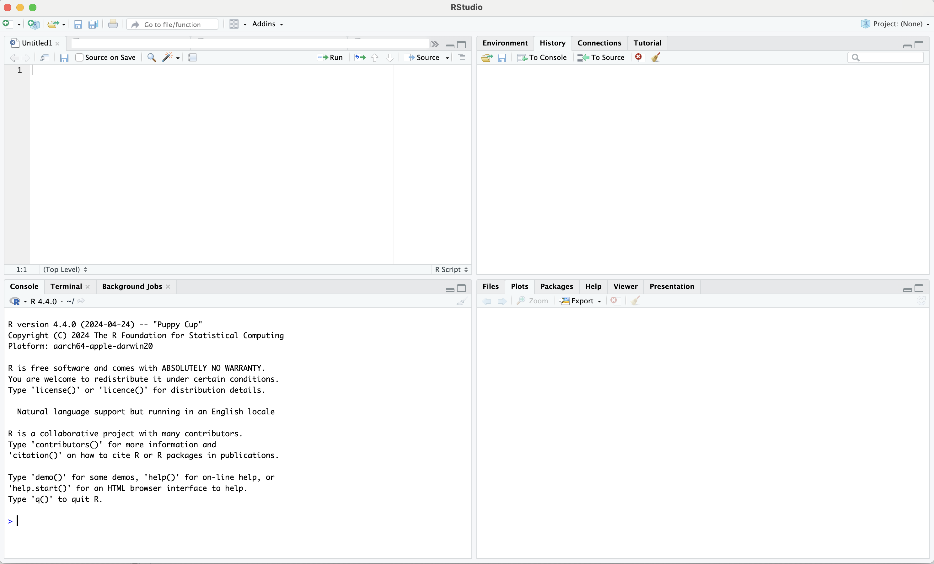
- Click on
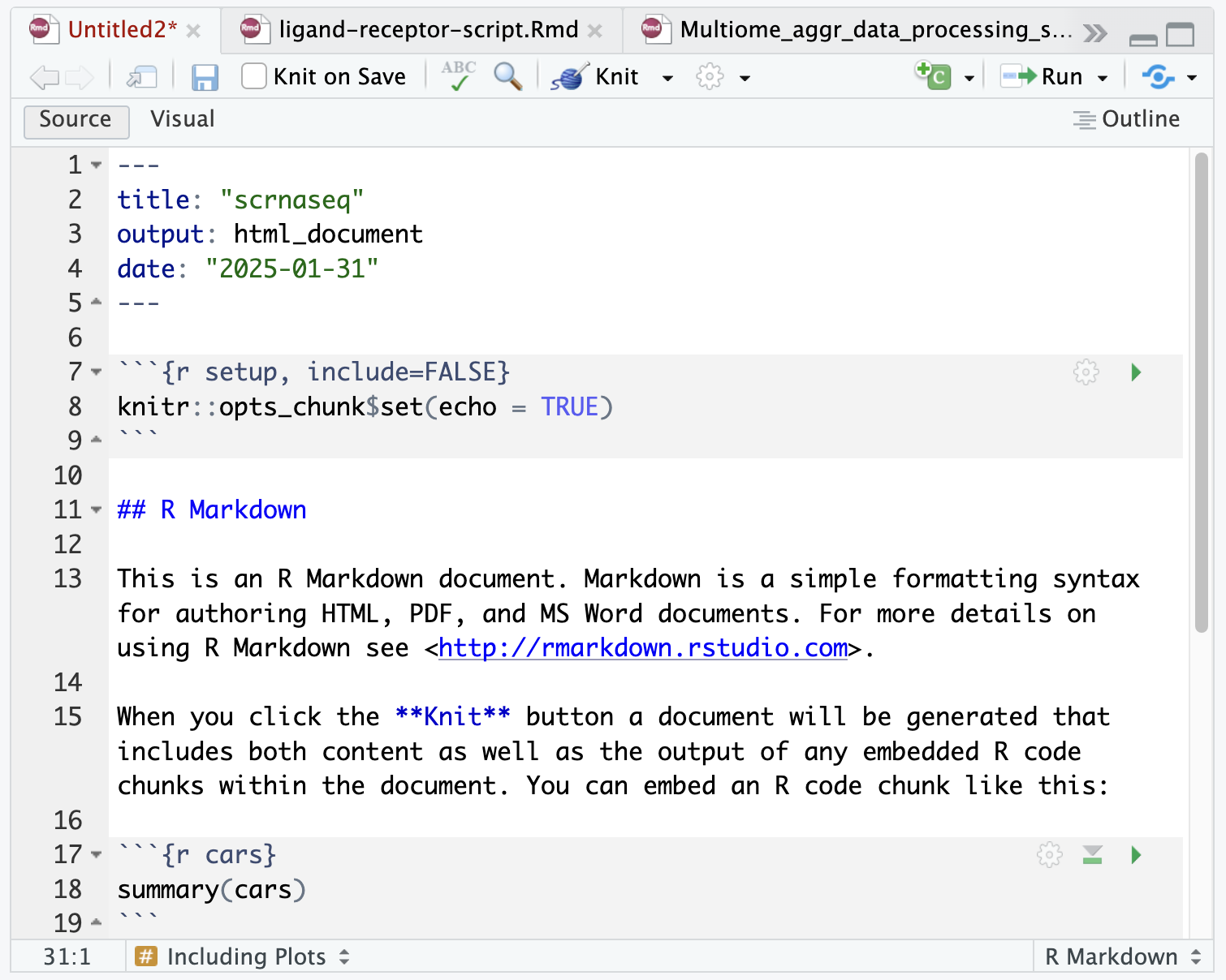
New File–>R Markdown...
- This is will open an
Untiltledfile on the top-left hand side.
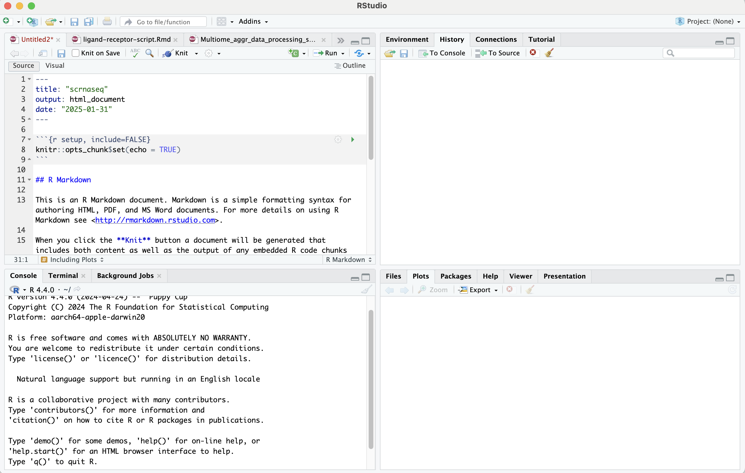
- Delete lines from 7 until 29 except first 5-6 lines.
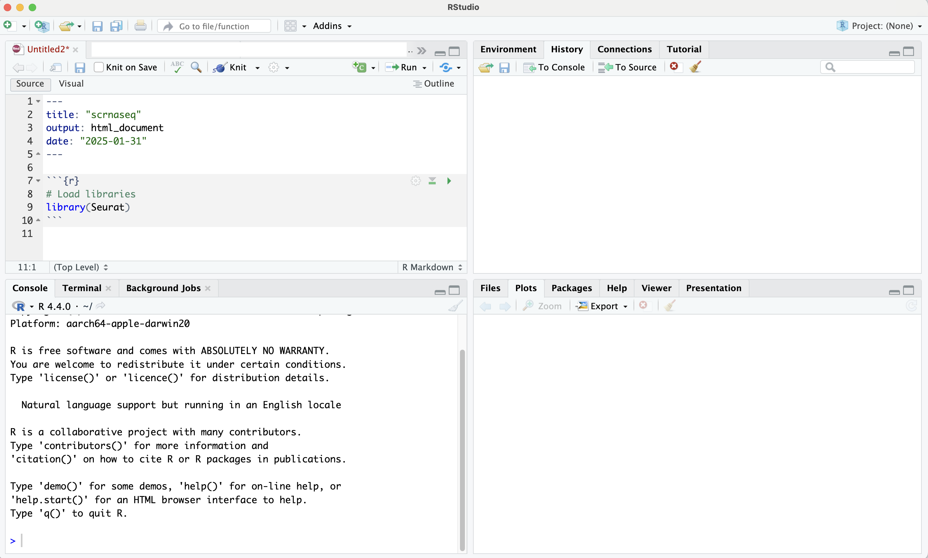
Load libraries
- Copy the line in your markdown document:
# load libraries
library(Seurat)
- Press the green arrow key on line 7 which says Run Current Chunk to load the Seurat library.
Setup the Seurat object
- We start by reading in the data. The
Read10X()function reads in the output of the cellranger pipeline from 10X, returning a unique molecular identified (UMI) count matrix. - The values in this matrix represent the number of molecules for each feature (i.e. gene; row) that are detected in each cell (column).
# Load the 1k mouse kidney dataset
dat2 <- Read10X(data.dir = "input/filtered_feature_bc_matrix/")
- We next use the count matrix to create a Seurat object.
# Initialize the Seurat object with the raw (non-normalized data).
dat2Obj <- CreateSeuratObject(counts = dat2, project = "1KmouseKidney", min.cells = 3, min.features = 200)

dat2Obj
## An object of class Seurat
## 18321 features across 1375 samples within 1 assay
## Active assay: RNA (18321 features, 0 variable features)
##  1 layer present: counts
QC and filtering cells for further analysis
- Seurat allows you to easily explore QC metrics and filter cells based on any user-defined criteria.
- These includes:
- The number of unique genes detected in each cell.
- Low-quality cells or empty droplets will often have very few genes
- Cell doublets or multiplets may exhibit an aberrantly high gene count
- The percentage of reads that map to the mitochondrial genome.
- Low-quality / dying cells often exhibit extensive mitochondrial contamination
- We calculate mitochondrial QC metrics with the
PercentageFeatureSet()function - We use the set of all genes starting with
MT-ormt-as a set of mitochondrial genes
- The number of unique genes detected in each cell.
# The [[ operator can add columns to object metadata.
dat2Obj[["percent.mt"]] <- PercentageFeatureSet(dat2Obj, pattern = "^mt-")
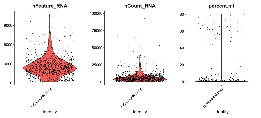
- To visualize QC metrics, we use
VlnPlot()function.
# Visualize QC metrics as a violin plot
VlnPlot(dat2Obj, features = c("nFeature_RNA", "nCount_RNA", "percent.mt"), ncol = 3)
Try using ^MT- as pattern. What do you get?
dat2Obj[["percent.mt"]] <- PercentageFeatureSet(dat2Obj, pattern = "^MT-")
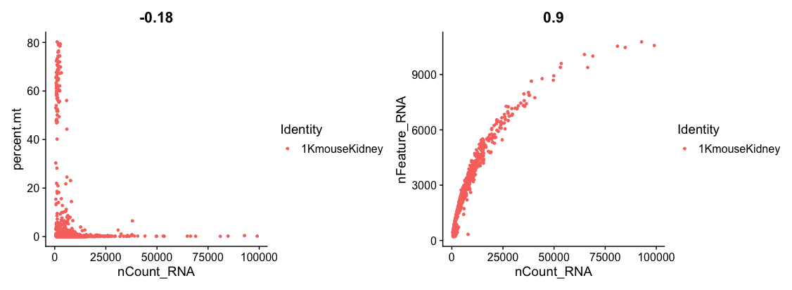
- Next, you can plot a FeatureScatter plot for visualising feature-feature relationships.
# Plot FeatureScatter plot
plot1 <- FeatureScatter(dat2Obj, feature1 = "nCount_RNA", feature2 = "percent.mt")
plot2 <- FeatureScatter(dat2Obj, feature1 = "nCount_RNA", feature2 = "nFeature_RNA")
plot1 + plot2
- Now, we will filter cells that have unique feature counts over 9000 or less than 200
- We filter cells that have >5% mitochondrial counts
dat2FilteredObj <- subset(dat2Obj, subset = nFeature_RNA > 200 & nFeature_RNA < 9000 &  percent.mt < 5)

dat2FilteredObj
# An object of class Seurat
# 18321 features across 1235 samples within 1 assay
# Active assay: RNA (18321 features, 0 variable features)
#  1 layer present: counts
Lets break it down:
nFeature_RNA > 200: Keeps cells that have more than 200 detected genes (features). This removes low-quality cells or empty droplets.Feature_RNA < 9000: Removes cells with too many detected genes, which might indicate doublets (two cells captured in one droplet).-
percent.mt < 5: Filters out cells where mitochondrial gene percentage is greater than 5%. High mitochondrial content often indicates damaged or dying cells. - With this command, the number of cells reduces to 1235.
Normalizing the data
- After removing unwanted cells from the dataset, the next step is to normalize the data.
- By default, we employ a global-scaling normalization method
LogNormalizethat normalizes the feature expression measurements for each cell by the total expression, multiplies this by a scale factor (10,000 by default), and log-transforms the result. - Normalized values are stored in
dat2NormalisedObj[["RNA"]]$data
dat2NormalisedObj <- NormalizeData(object = dat2FilteredObj, normalization.method = "LogNormalize", scale.factor = 10000)
- The use of
SCTransformreplaces the need to runNormalizeData,FindVariableFeatures, orScaleData.
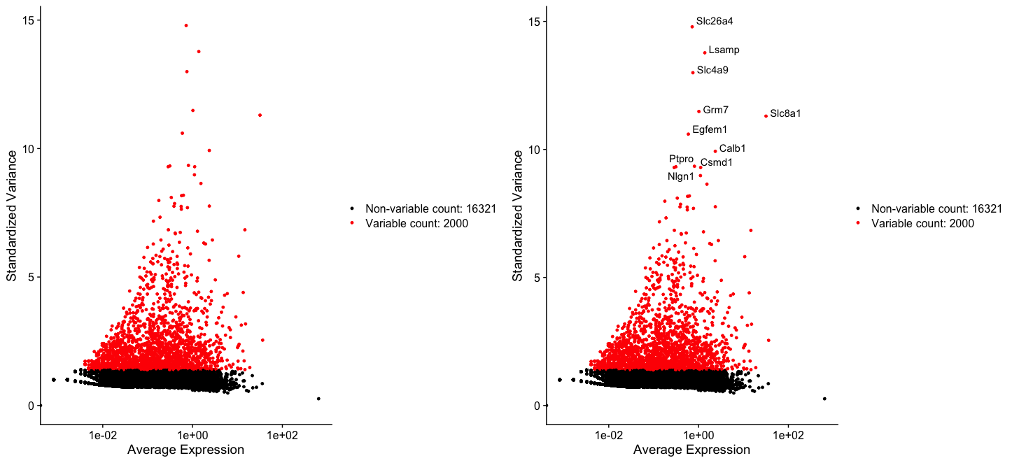
Identification of highly variable features (feature selection)
- We next calculate a subset of features (genes) that exhibit high cell-to-cell variation in the dataset.
- These are the features those are highly expressed in some cells, and lowly expressed in others.
- It has been found Brennecke et al. Nat Methods.2013 that focusing on these genes in downstream analysis helps to highlight biological signal in single-cell datasets.
dat2Normalised2Obj <- FindVariableFeatures(dat2NormalisedObj, selection.method = "vst", nfeatures = 2000)
top10 <- head(VariableFeatures(dat2Normalised2Obj), 10)
plot3 <- VariableFeaturePlot(dat2Normalised2Obj)
plot4 <- LabelPoints(plot = plot3, points = top10, repel = TRUE)
CombinePlots(plots = list(plot3, plot4))
Scaling the data
- The
ScaleDatafunction in Seurat is used to normalize and scale gene expression values across cells. - Additionally, it can regress out unwanted sources of variation, such as sequencing depth (
nUMI) or mitochondrial gene percentage (percent.mito), helping to remove technical artifacts. - By default, only variable features are scaled.
- But if you observe, in out script, we have used
rownames(dat2Normalised2Obj)which applies scaling to all genes which is stored inall.genesobject. - This is then applied to
ScaleDatafunction which usesall.genesas features for scaling.
all.genes <- rownames(dat2Normalised2Obj)
dat2ScaledObj <- ScaleData(object = dat2Normalised2Obj, features = all.genes)
How can I remove unwanted sources of variation
- To remove unwanted sources of variation from a single-cell dataset, such as "percent.mt", use "vars.to.regress" to include these:dat2ScaledObj <- ScaleData(object = dat2Normalised2Obj, features = all.genes, vars.to.regress = "percent.mt")
Perform linear dimensional reduction
- Next we perform PCA on the scaled data.
- By default, only the previously determined variable features are used as input, but can be defined using
featuresargument if you wish to choose a different subset.
dat2Scaled2Obj <- RunPCA(object = dat2ScaledObj, features = VariableFeatures(object = dat2ScaledObj), do.print = TRUE, ndims.print = 1:5, nfeatures.print = 5)
- This command uses only the highly variable genes (
VariableFeatures(object = dat2ScaledObj)) instead of all genes to reduce noise and improve clustering. do.print = TRUEprints the top genes contributing to each principal component (PC).pcs.print = 1:5displays the results for PC1 to PC5 (i.e., the first five principal components).- PC1 (Principal Component 1) is the most important axes of variation.
- PC2, PC3, PC4, etc. explain additional variation in the data.
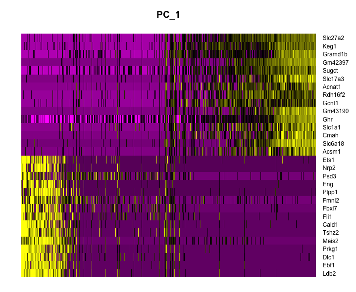
- Top Positive Genes (e.g., Ldb2, Ebf1, Prkg1, Meis2) are more highly expressed in one subset of cells.
- Top Negative Genes (e.g., Slc27a2, Keg1, Sugct) are more highly expressed in another subset.
- PC1 may capture a major biological signal, such as cell type differences.
- If PC2 separates a different cell population, it might represent a different biological process, like a cell cycle state or differentiation.
PC_ 1
Positive:  Ldb2, Ebf1, Dlc1, Prkg1, Meis2
Negative:  Slc27a2, Keg1, Gramd1b, Gm42397, Sugct
PC_ 2
Positive:  Slit2, Prdm16, Rgs6, Slc16a7, Me3
Negative:  Slc7a12, Aadat, Ldb2, Gm20400, Slc22a19
PC_ 3
Positive:  Sox5, Lama2, Kcnt2, Cfh, Svep1
Negative:  Adgrl4, Ptprb, Flt1, Emcn, St6galnac3
PC_ 4
Positive:  Chrm3, Slc7a12, Cd36, Mettl7a2, Gm30551
Negative:  Nox4, Bmp6, Bnc2, Slc34a1, Acsm2
PC_ 5
Positive:  Abca13, Fli1, Ldb2, Fbxl7, Sgms2
Negative:  Nphs1, Nphs2, Ptpro, Wt1os, Nebl
DimHeatmap()allows for easy exploration of the primary sources of heterogeneity in a dataset, and can be useful when trying to decide which PCs to include for further downstream analyses.
DimHeatmap(
    object = dat2Scaled2Obj,
    dims = 1,
    balanced = TRUE
)
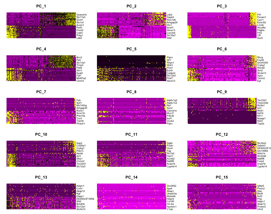
- Now, use dims 1 to 15 to plot 15 PCs to observe which PCs contribute to sources of variation in the dataset.
DimHeatmap(
    object = dat2Scaled2Obj,
    dims = 1:15,
    balanced = TRUE
)
Determining dimensionality
- After running PCA using
RunPCA(), you need to determine how many PCs to retain for clustering and downstream analysis. - One common method is using the Elbow Plot.
- The top principal components represents highest variations in the dataset.
- So, how many components should we choose to include? 10? 20? 100?
- In ‘Elbow plot’ it ranks principle components based on the percentage of variance explained by each one.
ElbowPlot(dat2Scaled2Obj)
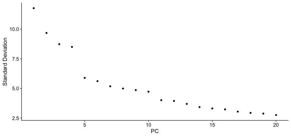
-
If we are considering going with the default settings with
ndims = 20, then we can clearly see that at the elbow point is at PC 11 which accounts for most variation in the dataset. -
However, if we choose to include
ndims = 50, then the elbow plot changes and includes 50 PCs.
ElbowPlot(dat2Scaled2Obj, ndims = 50)
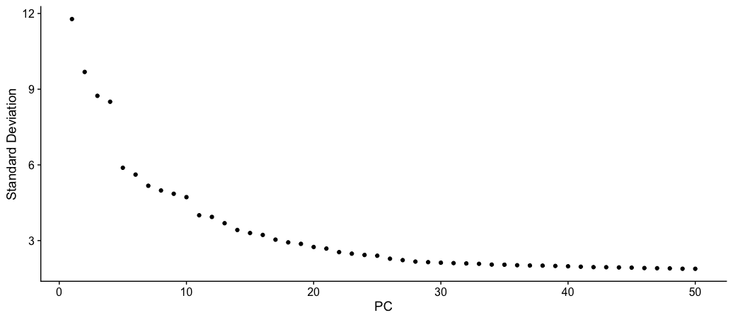
- Now, this gives us a much broader picture and also shows more PCs are contributing to variation beyond PC 11.
- With this plot, we can keep the value between PC 21-25.
- In this tutorial, I have chosen PC 25 to stretch the limit and include smaller variance. But the value of 21 will also work fine.
Clustering
- Seurat applies a graph-based clustering approach, called Shared Nearest Neighbors (SNN).
- How the SNN Score is Computed:
- If cell A’s neighbor list and cell B’s neighbor list share many cells, they are likely to be in the same cluster.
- The SNN score (edge weight) is higher if two cells have more shared neighbors.
- Example:
- Cell A’s neighbors: {B, C, D, E}
- Cell B’s neighbors: {A, C, D, F}
- Cell A and Cell B share: {C, D}
- SNN score = Number of shared neighbors / Minimum kNN list size
- SNN score = 2 / 4 = 0.5
- If two cells share many of their nearest neighbors, their SNN score is high, and they are more likely to belong to the same cluster.
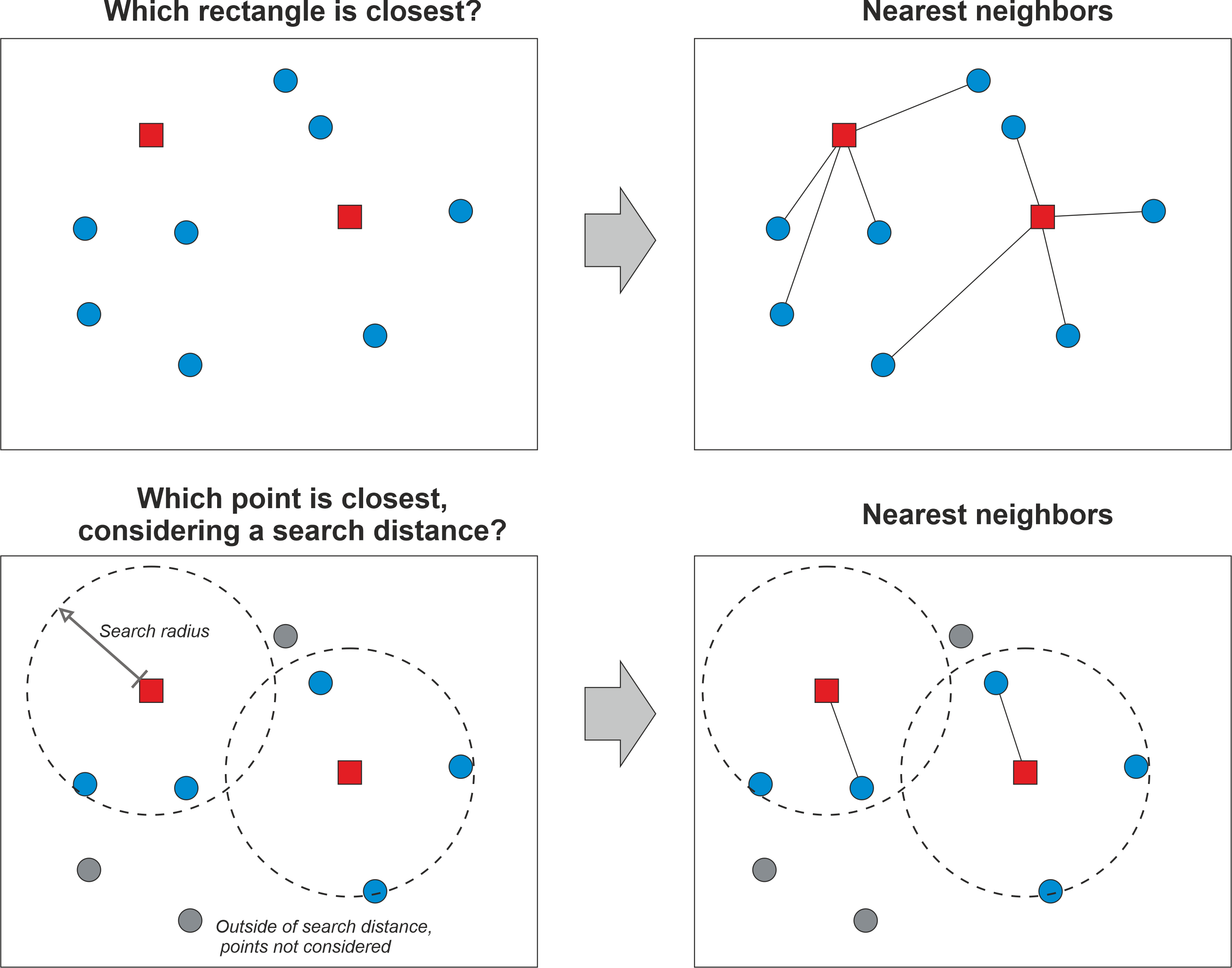
- So, the first step is performed using the
FindNeighbors()function, and takes as input the previously defined dimensionality of the dataset (first 25 PCs). - To cluster the cells, we next apply modularity optimization techniques such as the Louvain algorithm (default) or SLM to iteratively group cells together.
- The
FindClusters()function implements this procedure, and contains a resolution parameter that sets the ‘granularity’ of the downstream clustering, with increased values leading to a greater number of clusters.
Run the following commands:
seuratFindNeighbors <- FindNeighbors(
    dat2Scaled2Obj,
    reduction = "pca",
    dims = 1:25,
    do.plot = FALSE,
    graph.name = NULL,
    k.param = 30
)

seuratFindClusters <- FindClusters(object = seuratFindNeighbors)
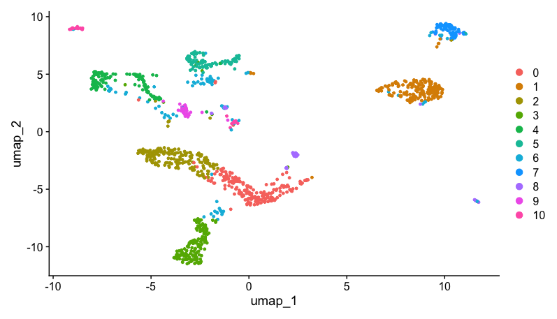
Non-linear dimensional reduction
- Seurat offers several non-linear dimensional reduction techniques, such as tSNE and UMAP, to visualize and explore these datasets.
- The goal of these algorithms is to learn underlying structure in the dataset, in order to place similar cells together in low-dimensional space.
- Therefore, cells that are grouped together within graph-based clusters determined above should co-localize on these dimension reduction plots.
dat2UMAP <- RunUMAP(seuratFindClusters, reduction = "pca", dims = 1:25, n.neighbors = 30L, min.dist = 0.3, seed.use = 123456L)
- If you see that we have used 25 PCs and
n.neighborsas 30 n.neighborsdefines the number of nearest neighbors considered when constructing the UMAP graph.- Larger values capture broader structures, while smaller values focus on finer details.
n.neighbors Value |
Effect on UMAP | When to Use? |
|---|---|---|
| Low (5-15) | Captures local structure, fine details | Small datasets, cluster refinement |
| Default (30) | Balanced between local and global structure | General use case |
| High (50-100) | Preserves global relationships, reduces fragmentation | Large datasets, broader clusters |
To generate UMAP, run the following command:
DimPlot(dat2UMAP, reduction = "umap")
Doublet detection and removal
- In scRNA-seq experiments, doublets are artifactual libraries generated from two cells.
- Doublets are defined when two or more cells are mistakenly treated as a single cell.
- They typically arise due to errors in cell sorting or capture, especially in droplet-based protocols involving thousands of cells.
- In this workshop, we will be using
DoubletFinder. - It is a tool used to detect and remove doublets (artificially merged cells) in scRNA-seq data.
- Below is a step-by-step guide to doublet detection and removal in Seurat using DoubletFinder.
Step 1: Install and Load Required Packages
remotes::install_github('chris-mcginnis-ucsf/DoubletFinder')
Once the package is installed, the load the library.
library(DoubletFinder)
Step 2: Parameter Sweeping for pK Selection
Sweep a range of parameters to find the optimal pK.
sweep.res.list <- paramSweep(dat2UMAP, PCs = 1:20, sct = TRUE)
sweep.stats <- summarizeSweep(sweep.res.list, GT = FALSE)
bcmvn <- find.pK(sweep.stats)
pk <- as.numeric(as.vector(bcmvn$pK)[which.max(bcmvn$BCmetric)])
paramSweep(): Tests multiple pK (parameter K) values using PCs 1 to 20.summarizeSweep(): Summarizes results into a dataframe.find.pK(): Finds the best pK using a “BCmetric” score.which.max(bcmvn$BCmetric): Selects the pK value with the highest BCmetric, as this gives the best separation between doublets and singlets.
Why do we need pK?
pKis a clustering resolution parameter that affects doublet detection.- A higher BCmetric means better performance of a given pK.
Step 3: Estimate the Expected Number of Doublets
annotations <- dat2UMAP@active.ident
homotypic.prop <- modelHomotypic(annotations)
nExp_poi <- round(0.076 * length(dat2UMAP@active.ident))
nExp_poi.adj <- round(nExp_poi * (1 - homotypic.prop))
modelHomotypic(annotations): Estimates homotypic doublets (cells of the same type that are mistakenly identified as a doublet).nExp_poi <- round(0.076 * length(p1tumorFilteredObj@active.ident)):- Uses 10X Genomics’ doublet rate formula: ~7.6% (0.076) × number of cells.
- This gives the expected number of doublets (
nExp_poi) in the dataset.
nExp_poi.adj <- round(nExp_poi * (1 - homotypic.prop))- Adjusts for homotypic doublets to avoid over-filtering.
Why adjust for homotypic proportion?
- If cells in a cluster are mostly from the same cell type, they might be misclassified as doublets.
- This adjustment prevents over-filtering of true biological clusters.
Step 4: Run DoubletFinder (First Pass)
seuratDoublet <- doubletFinder(dat2UMAP, PCs = 1:20, pN = 0.25, pK = pk,
                               nExp = nExp_poi, reuse.pANN = FALSE, sct = TRUE)
- This step assigns a probability score (
pANN) to each cell, indicating how likely it is a doublet.
Step 5: Prepare for Second Pass
pANN_String <- paste("pANN_0.25_", pk, "_", list(nExp_poi), sep="")
- Creates a string name for the pANN column, which stores doublet probability scores.
Step 6: Run DoubletFinder (Second Pass - Adjusted for Homotypic Doublets)
dat2UMAPDoublet <- doubletFinder(seuratDoublet, PCs = 1:10, pN = 0.25, pK = pk,
                                        nExp = nExp_poi.adj, reuse.pANN = pANN_String)
- The first pass identifies all doublets.
- The second pass refines the classification by removing homotypic doublets.
Step 7: Append doublets column in metadata
# Use this format: DF.classifications_pN_pk_nExp_poi

# Find out pk value
print(pk)

# Find out nExp_poi value
print(nExp_poi)

# Replace the DF.classifications_pN_pk_nExp_poi with the above values

# For example, if pk is 0.24 and nExp_poi is 134, then execute the following command

classificationsCol <- dat2UMAPDoublet@meta.data["DF.classifications_0.25_0.24_134"]

dat2UMAPDoublet@meta.data[,"DF_hi.lo"] <- classificationsCol[1]
- Now, construct a UMAP displaying the Doublets and Singlets.
- You can also generate Violin plot displaying the same information.
Remove doublets and pre-process singlets
Remove the doublets and select Singlets by performing the following command:
dat2UMAPSinglets <- subset(dat2UMAPDoublet, subset = DF_hi.lo == "Singlet")
Once the doublets are removed and singlets are selected, then re-run the following steps as performed above:
singletsNormalisedObj <- NormalizeData(object = dat2UMAPSinglets, normalization.method = "LogNormalize", scale.factor = 10000)
singletsNormalised2Obj <- FindVariableFeatures(singletsNormalisedObj, selection.method = "vst", nfeatures = 2000)
all.genes <- rownames(singletsNormalised2Obj)
singletsScaledObj <- ScaleData(object = singletsNormalised2Obj, features = all.genes)
singletsScaled2Obj <- RunPCA(object = singletsScaledObj, features = VariableFeatures(object = singletsScaledObj), do.print = TRUE, ndims.print = 1:5, nfeatures.print = 5)
ElbowPlot(singletsScaled2Obj, ndims = 50)
seuratFindNeighbors <- FindNeighbors(
    singletsScaled2Obj,
    reduction = "pca",
    dims = 1:25,
    do.plot = FALSE,
    graph.name = NULL,
    k.param = 30
)
singletsFindClusters <- FindClusters(object = singletsFindNeighbors)
singletsUMAP <- RunUMAP(singletsFindClusters, reduction = "pca", dims = 1:25, n.neighbors = 30L, min.dist = 0.3, seed.use = 123456L)
Once the pre-processing steps are finished, construct the UMAP using the DimPlot function.
DimPlot(singletsUMAP, reduction = "umap")
Data Visualisation
- There are several data visualisation methods and functions in Seurat which are used for visualising marker feature expression.
- This can be achieved using:
FeaturePlot()DotPlot()VlnPlot()RidgePlot()DimPlot()DoHeatmap()
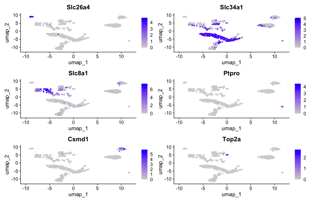
FeaturePlot function
- The
FeaturePlot()function in Seurat is used to visualize the expression of one or more genes (features) on a UMAP. - It helps in identifying the spatial distribution of gene expression across clusters or cell populations.
FeaturePlot(dat2UMAP, features = c("Slc26a4", "Slc34a1", "Slc8a1", "Ptpro", "Csmd1", "Top2a"))
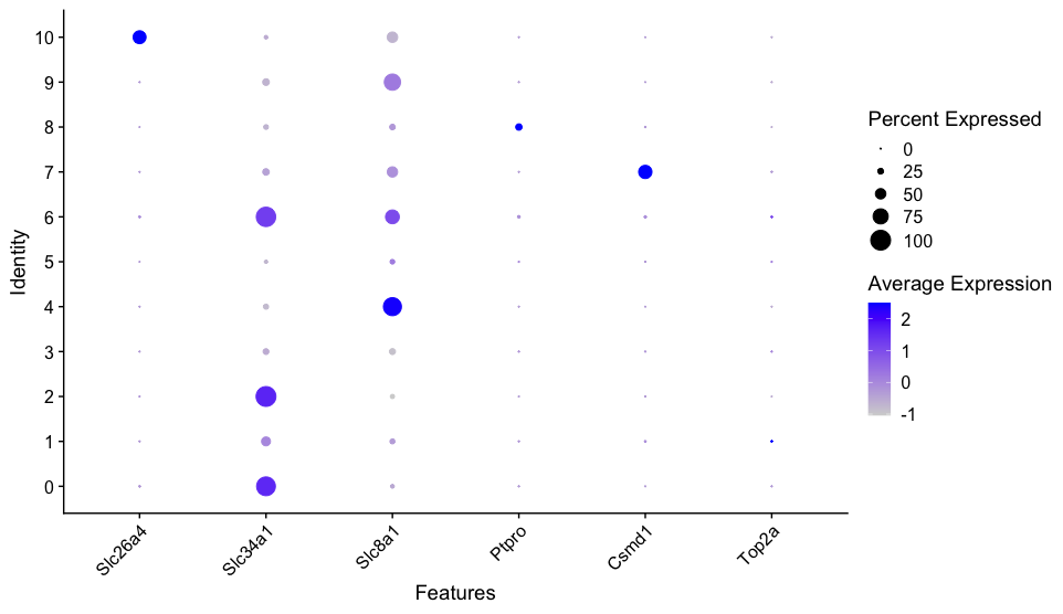
DotPlot function
- The
DotPlot()function in Seurat is used to visualize the expression levels of multiple genes across different clusters in a dot plot format. - It is particularly useful for comparing marker gene expression across cell clusters and assigning cell types.
genes = c("Slc26a4", "Slc34a1", "Slc8a1", "Ptpro", "Csmd1", "Top2a")
DotPlot(dat2UMAP, features = genes) + RotatedAxis()
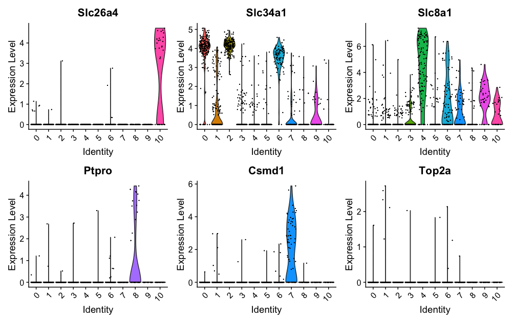
VlnPlot function
- The
VlnPlot()function in Seurat creates violin plots to visualize the distribution of gene expression levels across different clusters or groups of cells. - It helps in identifying differences in gene expression between clusters.
genes = c("Slc26a4", "Slc34a1", "Slc8a1", "Ptpro", "Csmd1", "Top2a")
VlnPlot(dat2UMAP, features = genes)
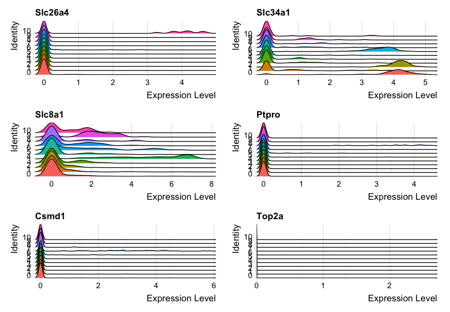
RidgePlot function
- The
RidgePlot()function in Seurat generates ridge plots to visualize the distribution of gene expression across different clusters or groups of cells. - It is useful for comparing the expression levels of genes in different cell populations.
genes = c("Slc26a4", "Slc34a1", "Slc8a1", "Ptpro", "Csmd1", "Top2a")
RidgePlot(dat2UMAP, features = genes, ncol = 2)
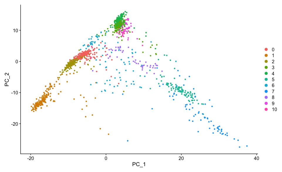
DimPlot function
- The
DimPlot()function in Seurat is used to visualize cells in a reduced dimensional space (e.g., UMAP, t-SNE, or PCA) and color them based on their cluster identity or metadata attributes. - It is useful for identifying and interpreting cell populations in single-cell RNA-seq analysis.
Syntax:
DimPlot(object, reduction = "umap", group.by = "ident", label = TRUE, pt.size = 1)
For example-
DimPlot(dat2UMAP, reduction = "pca")
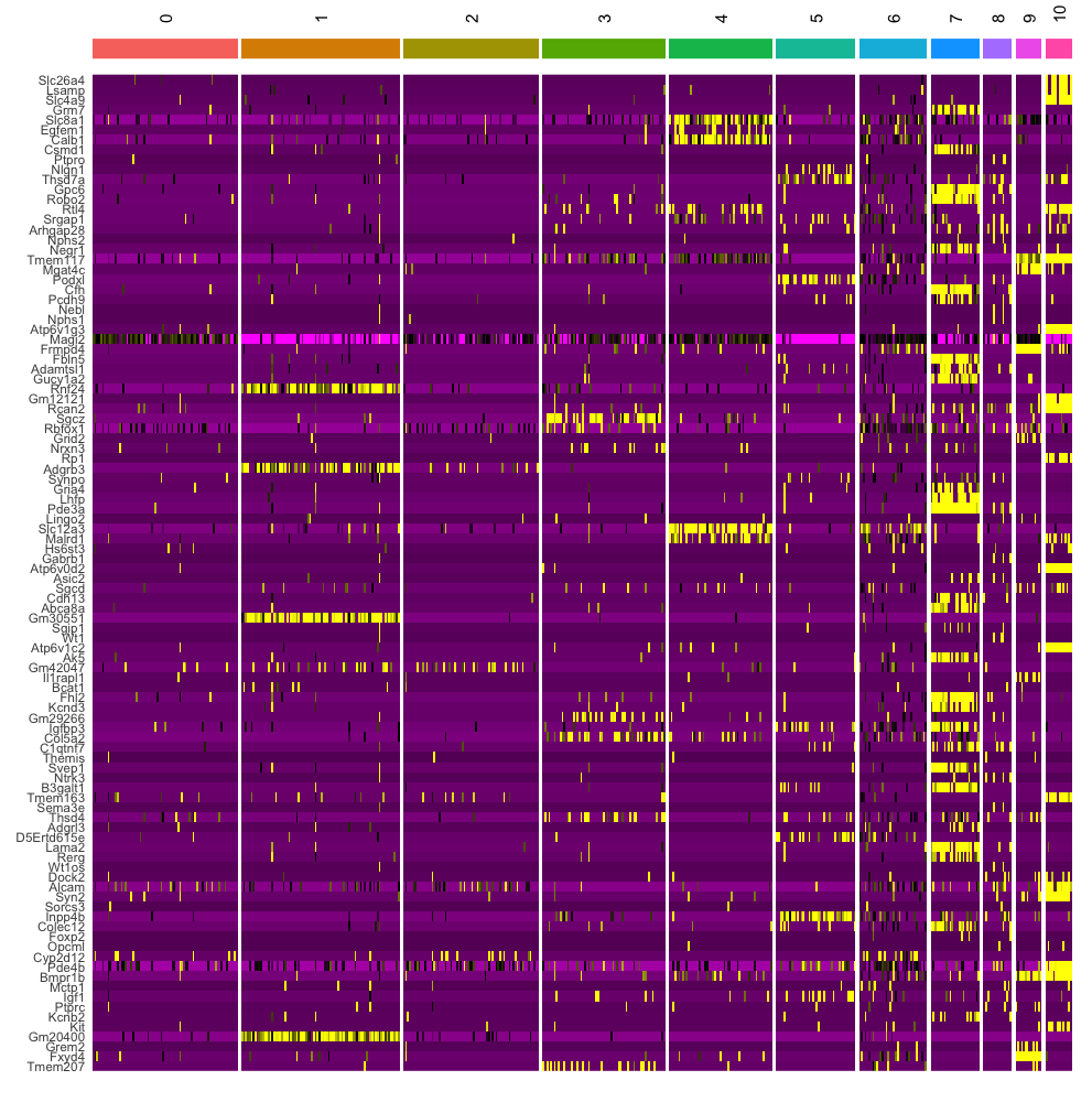
DoHeatmap function
- The
DoHeatmap()function in Seurat is used to generate a heatmap of gene expression across different cell clusters or groups. - It is particularly useful for visualizing the expression patterns of top marker genes across clusters.
DoHeatmap(dat2UMAP, features = VariableFeatures(dat2UMAP)[1:100], cells = 1:500, size = 4,
          angle = 90) + NoLegend()