Single Cell RNAseq Data Processing & Analysing Course

Day 3 - Analysing scRNAseq data in Seurat

Recap from Day 2

On 25th Feb, we covered:
- How to load cellranger data in RStudio.
- How to process scRNAseq data in Seurat.
  - Loading and creating seurat object
  - Generating QC metrics
  - Filtering data
  - Normalising data
  - Identifying highly variable genes
  - Scaling data
  - Performing Principal Component Analysis
  - Finding clusters (Clustering)
  - Visualising clusters using UMAP
  - Other visualisation functions to create plots for identifying differences in gene expression between clusters.
Today we will cover:
- Integrating single-cell datasets.
- Differential Gene Expression analysis and marker selection.
- Cell-type annotation using CellMarker.

scRNAseq Data Integration

Integration of single-cell sequencing datasets, for example across experimental batches, donors, or conditions, is often an important step in scRNA-seq workflows.
Integrative analysis can help to match shared cell types and states across datasets, which can boost statistical power, and most importantly, facilitate accurate comparative analysis across datasets.

Experiment

Cancer NSCLC processed sequencing data have been taken from GEO database (GSE117570).
4 early‐stage non‐small cell lung cancer (NSCLC) patients.
The Cell Ranger Single Cell Software Suite v.2.0.1 was used to perform sample de‐multiplexing, alignment, filtering, and UMI counting.
Paper reference: Qianqian et al. Cancer Medicine. 2019
Input files:
- Patient 1 - Normal
  - GSM3304008_P1_Normal_processed_data.txt
- Patient 1 - Tumor
  - GSM3304007_P1_Tumor_processed_data.txt
- Patient 2 - Normal
  - GSM3304010_P2_Normal_processed_data.txt
- Patient 2 - Tumor
  - GSM3304009_P2_Tumor_processed_data.txt
- Patient 3 - Normal
  - GSM3304012_P3_Normal_processed_data.txt
- Patient 3 - Tumor
  - GSM3304011_P3_Tumor_processed_data.txt
- Patient 4 - Normal
  - GSM3304014_P4_Normal_processed_data.txt
- Patient 4 - Tumor
  - GSM3304013_P4_Tumor_processed_data.txt

Setup and QC

Create a script called “NSCLC_dataset.Rmd” by following the instructions as instructed on Day-2.
Set the working directory to the bin folder where the script named “NSCLC_dataset.Rmd” will be stored. Setting up working directory:

setwd(/path/to/your/bin)

Load libraries:

library(Seurat)
library(DoubletFinder)

Load all the datasets:

# Loading P1 Tumor processed data

data <- read.table("input/GSM3304007_P1_Tumor_processed_data.txt",row.names = 1,header = T)
data1 <- data[-1]
p1tumor <- CreateSeuratObject(counts = data1, project = "GSM3304007")

# Loading P1 Normal processed data

data <- read.table("input/GSM3304008_P1_Normal_processed_data.txt",row.names = 1,header = T)
data1 <- data[-1]
p1normal <- CreateSeuratObject(counts = data1, project = "GSM3304008")

# Loading P2 Tumor processed data

data <- read.table("input/GSM3304009_P2_Tumor_processed_data.txt",row.names = 1,header = T)
data1 <- data[-1]
p2tumor <- CreateSeuratObject(counts = data1, project = "GSM3304009")

# Loading P2 Normal processed data

data <- read.table("input/GSM3304010_P2_Normal_processed_data.txt",row.names = 1,header = T)
data1 <- data[-1]
p2normal <- CreateSeuratObject(counts = data1, project = "GSM3304010")

# Loading P3 Tumor processed data

data <- read.table("input/GSM3304011_P3_Tumor_processed_data.txt",row.names = 1,header = T)
data1 <- data[-1]
p3tumor <- CreateSeuratObject(counts = data1, project = "GSM3304011")

# Loading P3 Normal processed data

data <- read.table("input/GSM3304012_P3_Normal_processed_data.txt",row.names = 1,header = T)
data1 <- data[-1]
p3normal <- CreateSeuratObject(counts = data1, project = "GSM3304012")

# Loading P4 Tumor processed data

data <- read.table("input/GSM3304013_P4_Tumor_processed_data.txt",row.names = 1,header = T)
data1 <- data[-1]
p4tumor <- CreateSeuratObject(counts = data1, project = "GSM3304013")

# Loading P4 Normal processed data

data <- read.table("input/GSM3304014_P4_Normal_processed_data.txt",row.names = 1,header = T)
data1 <- data[-1]
p4normal <- CreateSeuratObject(counts = data1, project = "GSM3304014")

Add percentage of reads that map to mitochondrial genome

p1tumor[["percent.mt"]] <- PercentageFeatureSet(p1tumor, pattern = "^MT-")
p1normal[["percent.mt"]] <- PercentageFeatureSet(p1normal, pattern = "^MT-")
p2tumor[["percent.mt"]] <- PercentageFeatureSet(p2tumor, pattern = "^MT-")
p2normal[["percent.mt"]] <- PercentageFeatureSet(p2normal, pattern = "^MT-")
p3tumor[["percent.mt"]] <- PercentageFeatureSet(p3tumor, pattern = "^MT-")
p3normal[["percent.mt"]] <- PercentageFeatureSet(p3normal, pattern = "^MT-")
p4tumor[["percent.mt"]] <- PercentageFeatureSet(p4tumor, pattern = "^MT-")
p4normal[["percent.mt"]] <- PercentageFeatureSet(p4normal, pattern = "^MT-")

Visualise QC metrics as violin plots

VlnPlot(p1tumor, features = c("nFeature_RNA", "nCount_RNA", "percent.mt"), ncol = 3)
VlnPlot(p1normal, features = c("nFeature_RNA", "nCount_RNA", "percent.mt"), ncol = 3)
VlnPlot(p2tumor, features = c("nFeature_RNA", "nCount_RNA", "percent.mt"), ncol = 3)
VlnPlot(p2normal, features = c("nFeature_RNA", "nCount_RNA", "percent.mt"), ncol = 3)
VlnPlot(p3tumor, features = c("nFeature_RNA", "nCount_RNA", "percent.mt"), ncol = 3)
VlnPlot(p3normal, features = c("nFeature_RNA", "nCount_RNA", "percent.mt"), ncol = 3)
VlnPlot(p4tumor, features = c("nFeature_RNA", "nCount_RNA", "percent.mt"), ncol = 3)
VlnPlot(p4normal, features = c("nFeature_RNA", "nCount_RNA", "percent.mt"), ncol = 3)

Now, filter cells. The first one has been done for you.

p1tumorFilteredObj <- subset(p1tumor, subset = nFeature_RNA > 200 & nFeature_RNA < 4000 &  percent.mt < 10)

Normalization, Scaling and Dimensional Reduction

Once the samples are filtered, then run the following steps for each sample in the iteration:

# Define the sample names
samples <- c("p1tumor", "p1normal", "p2tumor", "p2normal", "p3tumor", "p3normal", "p4tumor", "p4normal")

# Loop through each sample
for (sample in samples) {
  
  # Get the original Seurat object dynamically
  seurat_obj <- get(paste0(sample, "FilteredObj"))
  
  normalized_obj <- NormalizeData(object = seurat_obj, normalization.method = "LogNormalize", scale.factor = 10000)
  
  normalized2_obj <- FindVariableFeatures(normalized_obj, selection.method = "vst", nfeatures = 2000)
  
  all_genes <- rownames(normalized2_obj)
  scaled_obj <- ScaleData(object = normalized2_obj, features = all_genes)
  
  scaled2_obj <- RunPCA(object = scaled_obj, features = VariableFeatures(object = scaled_obj), 
                        ndims.print = 1:5, nfeatures.print = 5)
  
  ElbowPlot(scaled2_obj, ndims = 50)
  
  neighbors_obj <- FindNeighbors(scaled2_obj, reduction = "pca", dims = 1:25, k.param = 30)
  
  clusters_obj <- FindClusters(object = neighbors_obj)
  
  umap_obj <- RunUMAP(clusters_obj, reduction = "pca", dims = 1:25, n.neighbors = 30L, min.dist = 0.3, seed.use = 123456L)
  
  # Store results dynamically in the environment
  assign(paste0(sample, "NormalisedObj"), normalized_obj)
  assign(paste0(sample, "Normalised2Obj"), normalized2_obj)
  assign(paste0(sample, "ScaledObj"), scaled_obj)
  assign(paste0(sample, "Scaled2Obj"), scaled2_obj)
  assign(paste0(sample, "FindNeighbors"), neighbors_obj)
  assign(paste0(sample, "FindClusters"), clusters_obj)
  assign(paste0(sample, "UMAP"), umap_obj)
}

The results for each sample will be stored in its corresponding sample name + UMAP. For example, if you would like to access the object for p3tumor, the results is stored in p3tumorUMAP. For p4normal, the object is p4normalUMAP, and so on.

Doublet removal

Doublet identification

The next step is to identify doublets in the datasets. For this we will be using DoubletFinder tool in R.
Follow the steps as mentioned to identify and label the cells as Singlet or Doublet.

Run the loop to generate sampleName+FilteredDoublet file for every sample:

# Define the sample names
samples <- c("p1tumor", "p1normal", "p2tumor", "p2normal", "p3tumor", "p3normal", "p4tumor", "p4normal")

# Loop through each sample
for (sample in samples) {
  
  # Retrieve the filtered Seurat object dynamically
  seurat_obj <- get(paste0(sample, "UMAP"))
  
  # Perform parameter sweep
  sweep_res_list <- paramSweep(seurat_obj, PCs = 1:20, sct = TRUE)
  sweep_stats <- summarizeSweep(sweep_res_list, GT = FALSE)
  bcmvn <- find.pK(sweep_stats)
  pk <- as.numeric(as.vector(bcmvn$pK)[which.max(bcmvn$BCmetric)])
  
  # Calculate expected doublet proportion
  annotations <- seurat_obj@active.ident
  homotypic_prop <- modelHomotypic(annotations)
  nExp_poi <- round(0.076 * length(seurat_obj@active.ident))
  nExp_poi_adj <- round(nExp_poi * (1 - homotypic_prop))
  
  # Run DoubletFinder
  seuratDoublet <- doubletFinder(seurat_obj, PCs = 1:20, pN = 0.25, pK = pk, nExp = nExp_poi, reuse.pANN = FALSE, sct = TRUE)
  
  # Create pANN string
  pANN_String <- paste("pANN_0.25_", pk, "_", list(nExp_poi), sep = "")
  
  # Run DoubletFinder again with adjusted nExp
  seuratDoubletFinal <- doubletFinder(seuratDoublet, PCs = 1:10, pN = 0.25, pK = pk, nExp = nExp_poi_adj, reuse.pANN = pANN_String)
  
  # Extract classification column
  classCol <- paste("DF.classifications_0.25_", pk, "_", list(nExp_poi), sep = "")
  classificationsCol <- seuratDoubletFinal@meta.data[grepl(classCol, colnames(seuratDoubletFinal@meta.data))]
  
  # Assign doublet classification column
  seuratDoubletFinal@meta.data[,"DF_hi.lo"] <- classificationsCol[[1]]
  
  # Save the final object
  saveRDS(seuratDoubletFinal, paste0("output/", sample, "FilteredDoublet.rds"))
  
  # Store the processed object dynamically in the environment
  assign(paste0(sample, "FilteredDoublet"), seuratDoubletFinal)
}

This will generate doublet marked objects for all samples.

Singlet selection and doublet removal

In the next step, we use subset function in R to select Singlet and filter Doublet cells from the dataset.
This is iterated for all the samples.

p1tumorSinglets <- subset(p1tumorFilteredDoublet, subset = DF_hi.lo == "Singlet")
p1normalSinglets <- subset(p1normalFilteredDoublet, subset = DF_hi.lo == "Singlet")
p2tumorSinglets <- subset(p2tumorFilteredDoublet, subset = DF_hi.lo == "Singlet")
p2normalSinglets <- subset(p2normalFilteredDoublet, subset = DF_hi.lo == "Singlet")
p3tumorSinglets <- subset(p3tumorFilteredDoublet, subset = DF_hi.lo == "Singlet")
p3normalSinglets <- subset(p3normalFilteredDoublet, subset = DF_hi.lo == "Singlet")
p4tumorSinglets <- subset(p4tumorFilteredDoublet, subset = DF_hi.lo == "Singlet")
p4normalSinglets <- subset(p4normalFilteredDoublet, subset = DF_hi.lo == "Singlet")

Normalization and finding variable features

In the next step, simply create a list called sample_list which stores all the samples.

sample_list <- list()
sample_list[["p1tumorSinglets"]] <- p1tumor
sample_list[["p1normalSinglets"]] <- p1normal
sample_list[["p2tumorSinglets"]] <- p2tumor
sample_list[["p2normalSinglets"]] <- p2normal
sample_list[["p3tumorSinglets"]] <- p3tumor
sample_list[["p3normalSinglets"]] <- p3normal
sample_list[["p4tumorSinglets"]] <- p4tumor
sample_list[["p4normalSinglets"]] <- p4normal

Once the samples are added to the list, run NormalizeData and FindVariableFeatures functions to perform normalization and finding variable features using VST and nfeatures=2000.
Interate this step over all the samples in the sample_list.

for (i in 1:length(sample_list)) {
  sample_list[[i]] <- NormalizeData(sample_list[[i]], normalization.method = "LogNormalize", scale.factor = 10000)
  sample_list[[i]] <- FindVariableFeatures(sample_list[[i]], selection.method = "vst", nfeatures = 2000, verbose = T)
}

Perform Integration of samples

We will not integrate data with 8 samples (2 conditions for each Patient).
First step is to find integration anchors.

Step 1: Finding Integration Anchors

sample_anchors <- FindIntegrationAnchors(object.list = sample_list, dims = 1:30)

This step identifies anchors (shared biological structures) across multiple datasets in sample_list to help correct batch effects.
It first selects highly variable genes (default = 2000 features).
It then runs canonical correlation analysis (CCA) to find common biological signals across datasets.
The parameter dims = 1:30 means that the first 30 principal components (PCs) are used to define the anchors.

Step 2: Integrating the Data

allsamples_seurat <- IntegrateData(anchorset = sample_anchors, dims = 1:30)

This step applies batch correction using the integration anchors found in Step 1.
It merges all datasets into a single Seurat object (allsamples_seurat), where only the 2000 most variable features are stored in the “integrated” assay.
The batch-corrected data is now stored in the “integrated” assay.

Step 3: Switching Back to RNA Assay

DefaultAssay(allsamples_seurat) <- "RNA"

Changes the active assay from “integrated” to “RNA”.
This is necessary for normalization, scaling, and differential expression analysis because “integrated” data should not be used for these steps.

Why It’s Needed:

The “integrated” assay is only useful for dimensionality reduction (PCA, UMAP), clustering, and visualization.
Gene expression comparisons (e.g., FindMarkers()) should be done on the “RNA” assay to retain true biological signal.

Step 4: Merging Layers

allsamples_seurat1 <- JoinLayers(allsamples_seurat)

This step merges different data layers within the Seurat object to ensure all layers are accessible.
Specifically, it merges:
- Raw expression data (RNA)
- Integrated (batch-corrected) data
- Any other assays or metadata layers
This is useful for downstream analysis where you might need access to both raw and batch-corrected data.

Adding sample annotations

The next step after merging the samples is to add the annotations to the seurat object.
These annotations can be:
- Sample annotations such as P1-Tumor, P1-Normal, etc.
- Sample types such as Tumor/Normal
- Patient info such as P1, P2, P3, P4
We will add these annotations in a for loop:

allsamples_seurat1$geo_ID <- Idents(allsamples_seurat1)

geoIDs <- c("GSM3304007", "GSM3304008", "GSM3304009", "GSM3304010", "GSM3304011", "GSM3304012", "GSM3304013", "GSM3304014")

allsamples_seurat1$sampleName <- Idents(allsamples_seurat1)

allsamples_seurat1$sampleName <- plyr::mapvalues(
    x = allsamples_seurat1$orig.ident, 
    from = c("GSM3304007", "GSM3304008", "GSM3304009", "GSM3304010", "GSM3304011", "GSM3304012", "GSM3304013", "GSM3304014"), 
    to = c("P1_Tumor", "P1_Normal", "P2_Tumor", "P2_Normal", "P3_Tumor", "P3_Normal", "P4_Tumor", "P4_Normal")
)

allsamples_seurat1$sampleType <- plyr::mapvalues(
    x = allsamples_seurat1$orig.ident, 
    from = c("GSM3304007", "GSM3304008", "GSM3304009", "GSM3304010", "GSM3304011", "GSM3304012", "GSM3304013", "GSM3304014"), 
    to = c("Tumor", "Normal", "Tumor", "Normal", "Tumor", "Normal", "Tumor", "Normal")
)

allsamples_seurat1$patientInfo <- plyr::mapvalues(
    x = allsamples_seurat1$orig.ident, 
    from = c("GSM3304007", "GSM3304008", "GSM3304009", "GSM3304010", "GSM3304011", "GSM3304012", "GSM3304013", "GSM3304014"), 
    to = c("P1", "P1", "P2", "P2", "P3", "P3", "P4", "P4")
)

Perform Data Scaling

We will be using all.genes to capture all genes for data scaling.

all.genes <- rownames(allsamples_seurat1)
allsamplesScaleData <- ScaleData(allsamples_seurat1, features = all.genes)

Perform linear dimensional reduction

Next we perform PCA on the scaled data.
We use variable features by default, in which case only the previously determined variable features are used as input.

allsamplesPCA <- RunPCA(object = allsamplesScaleData, features = VariableFeatures(object = allsamplesScaleData), do.print = TRUE, ndims.print = 1:5, nfeatures.print = 5)

Plot ElbowPlot to calculate number of PCs

Next, we plot Elbow plot by running ElbowPlot function to determine number of PCs which define highest variance in the datasets.
We create this plot with ndims = 50

ElbowPlot(allsamplesPCA, ndims = 50)

gui1

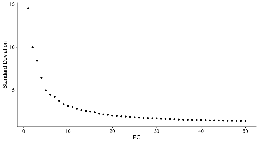
In this tutorial, I have chosen PC 20. Beyond this number, the variance seems to be stabilised and should be good enough to perform clustering.

Clustering

Next, we perform clustering by running FindNeighbors() and FindClusters() functions using the dimensionality determined by plotting ElbowPlot().
We take first 20 PCs as an input in this case.

allsamplesFN <- FindNeighbors(allsamplesPCA, reduction = "pca", dims = 1:25)
allsamplesFC <- FindClusters(object = allsamplesFN)

Non-linear dimensional reduction

In the next step, we run the RunUMAP() function to group the cells together constructing a UMAP plot.
Again, we use first 20 PCs.

allsamplesUMAP <- RunUMAP(allsamplesFC, reduction = "pca", dims = 1:25, verbose = T)

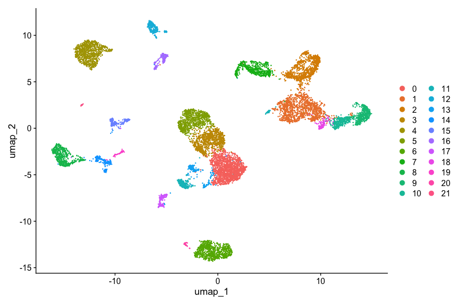
Generate UMAP plot

Before we generate the UMAP plot, it is important to change the default assay layer to integrated.

DefaultAssay(allsamplesUMAP) <- "integrated"
DimPlot(allsamplesUMAP, reduction = "umap")

gui1

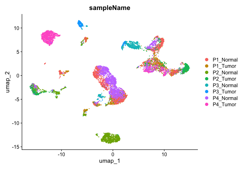
UMAP plot by sample name

To plot the UMAP by sampleName information stored in meta.data, use the following code:

DimPlot(allsamplesUMAP, reduction = "umap", group.by = "sampleName")

gui1

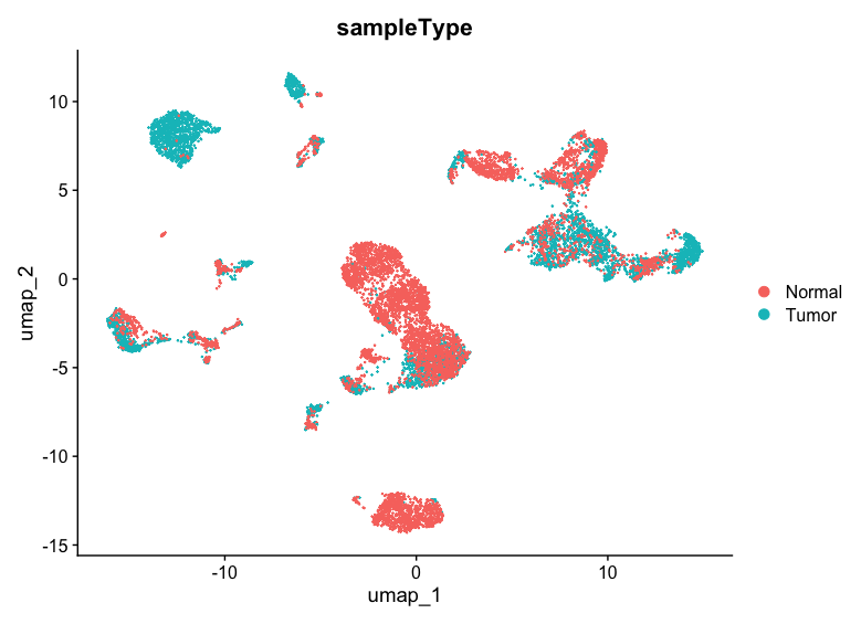
UMAP plot by sample type (Tumor/Normal)

To plot the UMAP by sampleType information stored in meta.data, use the following code:

DimPlot(allsamplesUMAP, reduction = "umap", group.by = "sampleType")

gui1

UMAP plot splitted by sample type (Tumor/Normal)

To plot the UMAP split-by sampleType information stored in meta.data, use the following code:

DimPlot(allsamplesUMAP, reduction = "umap", split.by = "sampleType")

gui1

Now, turn on the labels for each cluster.
How do you turn-on the labels ?
Which clusters are expressed in Tumor and Normal cells ?

Differential Gene Expression (DGE)

In Seurat, Differential Expression (DE) analysis is used to identify genes that are differentially expressed between different cell groups (clusters, conditions, or sample types).
Seurat provides several methods for performing DGE, primarily through the FindMarkers() and FindAllMarkers() functions.
For Example: If you would like to find all the markers for clusters 2, then you would run the following command:

cluster2.markers <- FindMarkers(allsamplesUMAP, ident.1 = 2)

Now, if you want to find all markers distinguishing cluster 5 from clusters 0 and 3, run the following command:

cluster5.markers <- FindMarkers(allsamplesUMAP, ident.1 = 5, ident.2 = c(0, 3))

List the top 5 markers which are expressed significantly in cluster 2.

head(cluster2.markers, n = 5)

If you want to find markers for every cluster compared to all remaining cells, then run the following command:

allsamples.markers <- FindAllMarkers(allsamplesUMAP)

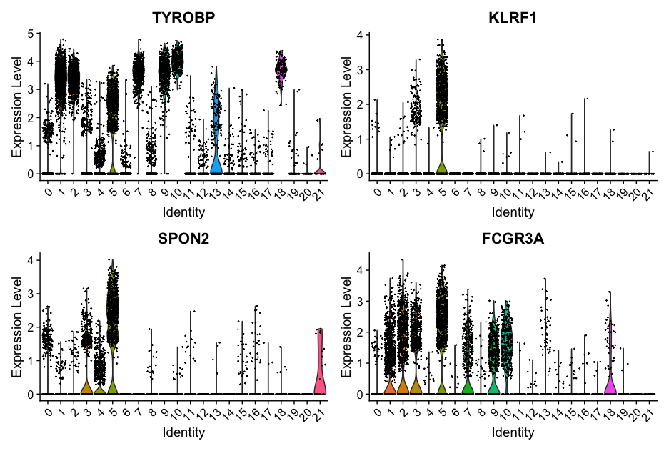
To plot the expression of genes expressed in cluster 5, run the following command:

VlnPlot(allsamplesUMAP, features = c("TYROBP", "KLRF1", "SPON2", "FCGR3A"), ncol = 2)

gui1

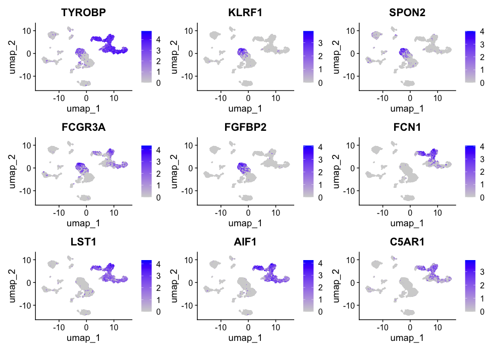
Now, to plot the expression of cluster 2 and 5 genes as feature plots, run the following command:

FeaturePlot(allsamplesUMAP, features = c("TYROBP", "KLRF1", "SPON2", "FCGR3A", "FGFBP2", "FCN1", "LST1", "AIF1", "C5AR1"))

gui1

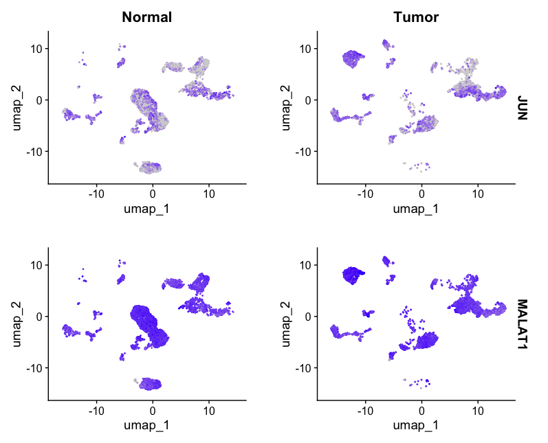
To plot the Feature plot by sampleType i.e Tumor/Normal for JUN1 and MALAT1 genes which are upregulated in the intratumoral epithelial cell, run the following command:

FeaturePlot(allsamplesUMAP, features = c("JUN", "MALAT1"), split.by = "sampleType")

gui1

Method 1: Cell Type Identification - Knowledge-based approach

-To identify and clssify the cell types, it is often recommended to obtain a list of well-established markers and assign these markers to the clusters in which they are primarily expressed.

Follow these steps for defining the celltypes:
Collect Cell Type Markers from Published Papers
- Search for scRNA-seq studies on similar tissue/cancer types.
- Extract well-established marker genes for different cell types.
- Example marker genes for common immune cells in NSCLC:
  - B cells → CD19, MS4A1
  - T cells → CD3D, CD3E, CD4, CD8A
  - Macrophages → CD68, CD163, MARCO
  - Epithelial cells → EPCAM, KRT19
  - Fibroblasts → COL1A1, DCN
  - Dendritic cells → CD1C, CLEC9A
Generate a FeaturePlot and DotPlot to Visualize Marker Expression
Fro example, the T-cell markers can be plotted using the following commands:

DefaultAssay(allsamplesUMAP) <- "RNA"

# T-cells
tcellmarkers <- c("CD3D", "CD3E", "CD3G", "CD4", "CD8A", "CD40")

FeaturePlot(allsamplesUMAP, features = tcellmarkers, pt.size = 0.5)
DotPlot(allsamplesUMAP, features = tcellmarkers, cols = c("blue", "red"), dot.scale = 8) + RotatedAxis()

In order to assign to assign the cell type, first create a copy of allsamplesUMAP object and call it as allsamplesUMAP1.
The Idents are replaced with the predicted celltype using the following commands:

allsamplesUMAP1 <- allsamplesUMAP
allsamplesUMAP1[["org.ident"]] <- Idents(object = allsamplesUMAP1)

allsamplesUMAP1 <- RenameIdents(object = allsamplesUMAP1, 
                                `0` = "T cells", 
                                `1` = "Macrophages", 
                                `2` = "M1 Macrophages",
                                `3` = "T cells",
                                `4` = "Epithelial cells",
                                `5` = "NK cells",
                                `6` = "Epithelial cells",
                                `7` = "Macrophages",
                                `8` = "Epithelial cells",
                                `9` = "M1 Macrophages",
                                `10` = "M1 Macrophages",
                                `11` = "NK cells",
                                `12` = "Epithelial cells",
                                `13` = "NK cells",
                                `14` = "Epithelial cells",
                                `15` = "Alveolar Type II (AT2) Cells",
                                `16` = "Fibroblasts",
                                `17` = "B cells",
                                `18` = "M2 Macrophages",
                                `19` = "Epithelial cells",
                                `20` = "Epithelial cells",
                                `21` = "Epithelial cells")

Plot the UMAP using the predicted celltype using the following command:

DimPlot(allsamplesUMAP1, reduction = "umap", label = TRUE, pt.size = 0.8)

Method 2: Cell Type Identification using CellMarker

CellMarker is a manually curated database human and mouse species.
Its manually curated over 100,000 published papers, 4124 entries including the cell marker information.
13,605 cell markers of 467 cell types in 158 human tissues/sub-tissues and 9148 cell makers of 389 cell types in 81 mouse tissues/sub-tissues were collected and deposited in CellMarker.
Paper Reference: CellMarker: a manually curated resource of cell markers in human and mouse.

For this dataset, we will be downloading the “Human cell markers” from CellMarker database.
Human Cell markers: download or visit the download page: download page
Other cell markers are as follows:
- Mouse cell markers: download
- Single cell markers: download
- All cell markers: download

Finding marker genes for NSCLC data in CellMarker database

Load the dataset in Rstudio. You will need to have readxl library installed.

install.packages("readxl")
library(readxl)

Once the library is installed and loaded, load the database using read_xlsx function.

cellMarkerDF <- read_xlsx("Cell_marker_Human.xlsx")

Type cellMarkerDF in the console to view the dataframe.

cellMarkerDF

We will now filter the rows based on target cancer type.
We are interested in viewing those markers expressed in NSCLC.
From the database, there are “non-small cell” and “lung cancer” types available.
Therefore we will be using these patterns to filter the dataframe to limit the markers to these cancer types.
You can add additional filter parameters such as “cell_type” column which contains two entries: “Normal cell” and “Cancer cell”

patterns <- c("non-small cell", "lung cancer")
filtered_df <- cellMarkerDF %>% 
  filter(grepl(paste(patterns, collapse = "|"), cancer_type, ignore.case = TRUE))

# Extract only the "cell_name", "marker" and "tissue_type" columns from the filtered_df dataframe
filtered_df1 <- filtered_df[,c("cell_name","marker","tissue_type")]

# Rename the "marker" column to "gene"
colnames(filtered_df1)[2] = "gene"

Filter the allsamples.markers to select only the markers which are differentially expressed with adjusted p_value less than or equal to 0.05.

allsamples.markers.sig <- allsamples.markers[allsamples.markers$p_val_adj <= 0.05, ]

Nxt, merge the two dataframes allsamples.markers.sig and filtered_df1 by gene column to append the cancer_type

allsamples.markers_sig_annot <- merge(allsamples.markers.sig, filtered_df1, by="gene", all.x=T, sort=F)

Get the markers expressed in a specific cluster, such as cluster 0.

cluster0_cellmarker <- allsamples.markers_sig_annot[which(allsamples.markers_sig_annot$cluster == 0),]

In order to assign the celltypes, an automated way is to define the celltypes for the NSCLC data and find out the frequency of each celltype in each cluster.

For example, to find out the frequency of the celltypes in Cluster 0, run the following loop:

# Define the cell types to search for
cell_types <- c("B cell", "T cell", "Macrophage", "Epithelial cell", "Monocyte", 
                "Myeloid cell", "Dendritic cell", "M1 macrophage", "M2 macrophage", 
                "Natural killer cell", "Fibroblast", "Plasma cell")

# Initialize an empty list to store counts
cell_type_counts <- list()

# Loop through each cell type and count occurrences
for (cell_type in cell_types) {
    count <- sum(grepl(cell_type, cluster0_cellmarker$cell_name, ignore.case = TRUE))
    cell_type_counts[[cell_type]] <- count
    print(paste(cell_type, "count:", count))
}

# Convert the list to a dataframe
cell_type_counts_df <- data.frame(Cell_Type = names(cell_type_counts), Count = unlist(cell_type_counts))

# Print the final counts
print(cell_type_counts_df)

This gives us the following table for Cluster 0:

Cell_Type	Count
B cell	8
T cell	5
Macrophage	14
Epithelial cell	5
Monocyte	2
Myeloid cel	5
Dendritic cell	2
M1 macrophage	2
M2 macrophage	3
Natural killer cell	1
Fibroblast	4
Plasma cell	2

Finally, assign the cell types in the same manner as in Method 1.