Day 4 - Cell-type Identification and Trajectory Analysis in Seurat
Recap from Day 3
- On 27th Feb, we covered:
- Integrating single-cell datasets.
- Differential Gene Expression analysis and marker selection.
- Cell-type annotation using CellMarker.
- Today we will cover:
- Cell-type annotation using SingleR.
- Trajectory analysis (pseudotime analysis) using monocle3
Cell-type annotation using SingleR
What is SingleR?
- SingleR is an automatic annotation method for single-cell RNA sequencing (scRNAseq) data.
- Given a reference dataset of samples (single-cell or bulk) with known labels, it labels new cells from a test dataset based on similarity to the reference.
- The burden of manually interpreting clusters and defining marker genes only has to be done once.
- This biological knowledge can be propagated to new datasets in an automated manner.
Using built-in references
- The easiest way to use SingleR is to annotate cells against built-in references.
- The
celldexR package provides access to several reference datasets.
General-purpose references
- Human primary cell atlas (HPCA): Publicly available microarray datasets derived from human primary cells.
- Blueprint/ENCODE: Bulk RNA-seq data for pure stroma and immune cells generated by Blueprint and ENCODE projects.
- Mouse RNA-seq: Collection of mouse bulk RNA-seq data sets downloaded from the gene expression omnibus.
Immune references
- Immunological Genome Project (ImmGen): Consists of microarray profiles of pure mouse immune cells.
- Database of Immune Cell Expression/eQTLs/Epigenomics (DICE): The
DICEreference consists of bulk RNA-seq samples of sorted cell populations. - Novershtern hematopoietic data: The Novershtern reference (previously known as Differentiation Map) consists of microarray datasets for sorted hematopoietic cell populations from GSE24759.
- Monaco immune data: The Monaco reference consists of bulk RNA-seq samples of sorted immune cell populations from GSE107011.
Downloading reference dataset
- Since the dataset we are working with is the NSCLC scRNAseq dataset, we will be working with HPCA dataset.
- To download the reference data, use the
fetchReference()function.
# Load the celldex package

library(celldex)

# Download the reference database

ref <- fetchReference("hpca", "2024-02-26")
SingleR requires the seurat object to be converted to SingleCellExperiment object. Therefore, we will be doing the conversion step at this point.
# Convert Seurat object to SingleCellExperiment object

allsamplesUMAP.SCE <- as.SingleCellExperiment(allsamplesUMAP)
Run the SingleR function to perform mapping of target dataset onto the reference dataset.
pred.allsamples <- SingleR(test = allsamplesUMAP.SCE, ref = ref, assay.type.test=1,
                           labels = ref$label.main)
What does SingleR function do ?
- It assigns cell types to individual cells by comparing their gene expression profiles to reference datasets with known cell type annotations.
- How
SingleRWorks:- Input Data: Takes a query dataset containing gene expression data for single cells.
- Reference Dataset: Uses a reference dataset with pre-annotated cell types from celldex, such as HumanPrimaryCellAtlasData.
- Correlation Analysis: Compares the gene expression of each cell in the query dataset to the reference profiles using Spearman correlation or other similarity measures.
- Scoring & Classification: Assigns the most likely cell type based on the highest similarity score.
- Fine-tuning: Iteratively refines the annotations by removing ambiguous labels and reassigning cells.
Type in pred.allsamples to see the output of the analysis:
print(pred.allsamples)
Now we will need to convert the row names to cell_ID column and will create a new dataframe with a name pred.allsamples.df and remove the row names from the dataframe.
pred.allsamples.df <- data.frame(cell_ID = row.names(pred.allsamples), pred.allsamples)
rownames(pred.allsamples.df) <- NULL
Next, select the cell_ID and labels columns and store the columns in a new dataframe.
pred.allsamples.df_labels <- pred.allsamples1.df[,c(1,ncol(pred.allsamples1.df)-2)]
Create a copy of allsamplesUMAP object and call it allsamplesUMAP1 so that any changes that are made does not affect the original object.
allsamplesUMAP1 <- allsamplesUMAP
Now, add cell_ID column to the allsamplesUMAP1 seurat object which is copied from the row names in the metadata.
allsamplesUMAP1@meta.data <- data.frame(cell_ID = row.names(allsamplesUMAP1@meta.data), allsamplesUMAP1@meta.data)
Also, create another column called predicted_cell_type column in the metadata of allsamplesUMAP1 object. Dont worry. The values in this column will get replaced with the predicted cell type values using output from SingleR analysis stored in the dataframe pred.allsamples.df_labels.
allsamplesUMAP1$predicted_cell_type <- allsamplesUMAP1$cell_ID
Create a vector cell_IDs and predicted celltypes.
prediction_ids <- pred.allsamples.df_labels$cell_ID
prediction_celltypes <- pred.allsamples.df_labels$labels
Now, run a for loop over the cell_IDs stored in pred.allsamples.df_labels dataframe and replace the IDs with the predicted celltypes. With every iteration of the cell_ID value, the cell_ID value gets replaced with the predicted celltype value.
for( i in 1:length(prediction_ids)) {

    print(prediction_ids[i])
    allsamplesUMAP1@meta.data["predicted_cell_type"][allsamplesUMAP1@meta.data["predicted_cell_type"] == prediction_ids[i]] <- prediction_celltypes[i]

}
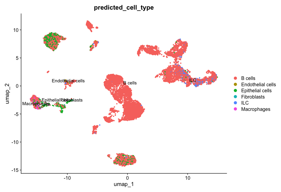
Plot the UMAP using the predicted_cell_type column stored in the meta.data:
DimPlot(allsamplesUMAP1, reduction = "umap", group.by = "predicted_cell_type", label = TRUE, pt.size = 0.8)
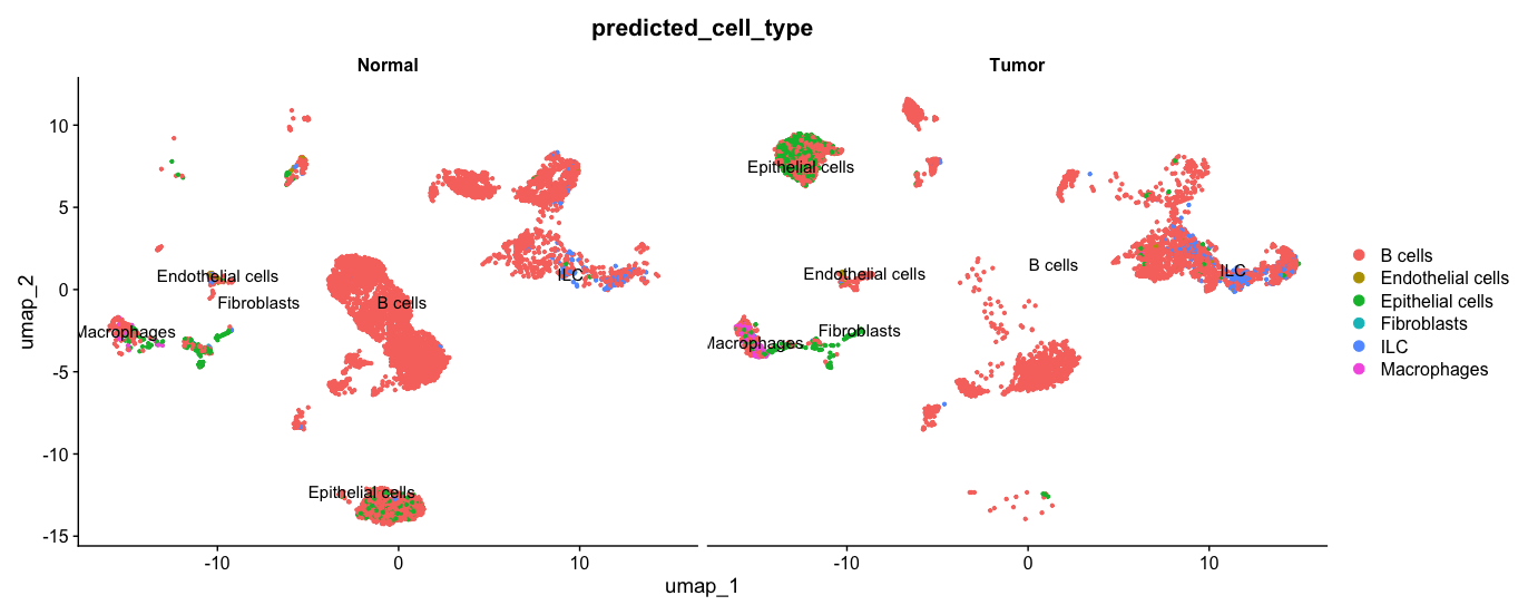
Plot the UMAP split-by sampleType column (Tumor/Normal):
DimPlot(allsamplesUMAP1, reduction = "umap", group.by = "predicted_cell_type", split.by = "sampleType", label = TRUE, pt.size = 0.8)
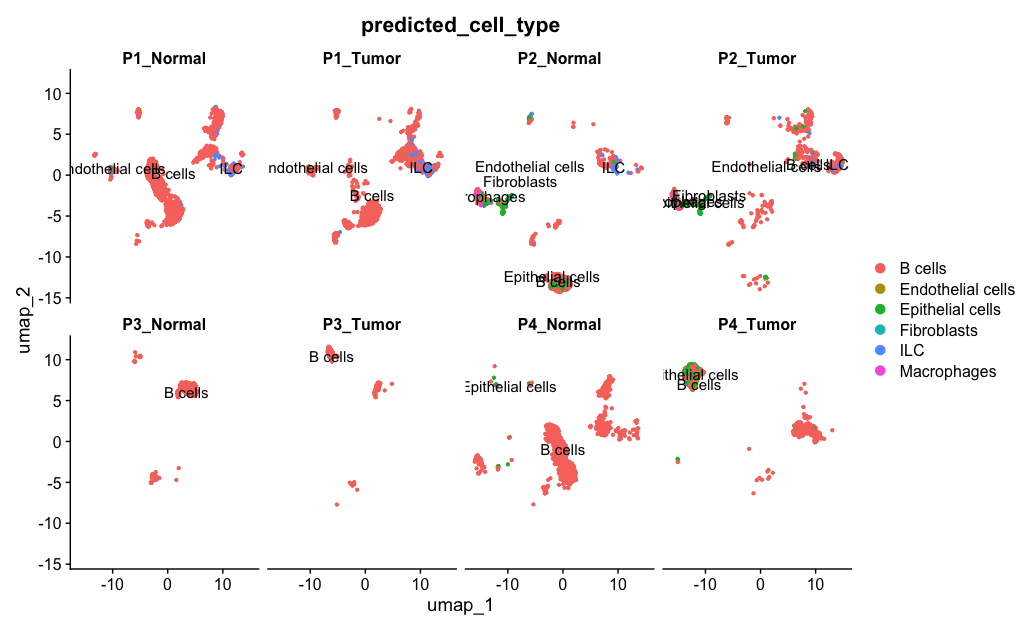
Further to the analysis, if we need to UMAP by sampleName (P1_Tumor, P1_Normal, P2_Tumor, P2_Normal, etc.), use the split.by parameter:
DimPlot(allsamplesUMAP1, reduction = "umap", group.by = "predicted_cell_type", split.by = "sampleName", label = TRUE, pt.size = 0.8, ncol = 4)
Trajectory analysis
- We will be using Monocle3 R package to perform trajectory analysis.
- In development, disease, and throughout life, cells transition from one state to another. Monocle 3 helps you discover these transitions.
- For this analysis, we will be using counts data from C.elegens species.
Load the monocle library
library(monocle3)
We will download the expression_matrix, cell_metadata and gene_annotation data.
expression_matrix <- readRDS(url("https://depts.washington.edu:/trapnell-lab/software/monocle3/celegans/data/packer_embryo_expression.rds"))
cell_metadata <- readRDS(url("https://depts.washington.edu:/trapnell-lab/software/monocle3/celegans/data/packer_embryo_colData.rds"))
gene_annotation <- readRDS(url("https://depts.washington.edu:/trapnell-lab/software/monocle3/celegans/data/packer_embryo_rowData.rds"))```
Now, create a new cell_data_set object using the new_cell_data_set() function.
cds <- new_cell_data_set(expression_matrix,
                         cell_metadata = cell_metadata,
                         gene_metadata = gene_annotation)
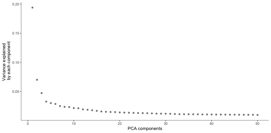
Pre-process the data
- Once the data is loaded, we need to pre-process the data in which the data will get normalized.
- We will just use the standard PCA method with
ndims = 50.
cds1 <- preprocess_cds(cds, num_dim = 50)
This will create an elbow plot similar to the one generated using Seurat.
plot_pc_variance_explained(cds1)
- The next step is to check for and remove batch effects in the data which are systematic differences in the transcriptome of cells measured in different experimental batches.
- These could be technical in nature, such as those introduced during the single-cell RNA-seq protocol, or biological.
cds2 <- align_cds(cds1, alignment_group = "batch", residual_model_formula_str = "~ bg.300.loading + bg.400.loading + bg.500.1.loading + bg.500.2.loading + bg.r17.loading + bg.b01.loading + bg.b02.loading")
- The function
align_cds()in Monocle3 is performing batch correction for cell_data_set (CDS) object. - The formula tells Monocle3 to remove unwanted variation due to specific technical or biological factors.
- The bg.*.loading terms likely represent confounding variables (e.g., sequencing depth, technical artifacts, or sample conditions).
- By including them in the residual model, Monocle3 accounts for their effects so they don’t dominate the biological signal.
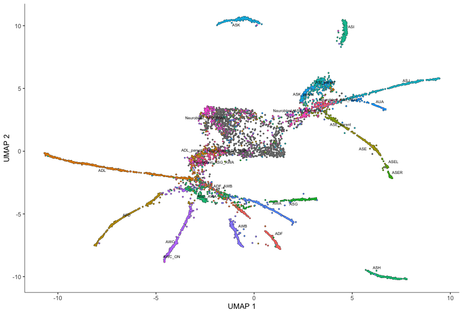
Once the data is aligned and unwanted variation is removed, then perform dimensionality reduction step using reduce_dimension() function.
cds3 <- reduce_dimension(cds2)
- Monocle 3 uses UMAP by default, as it is both faster and better suited for clustering and trajectory analysis.
- To plot the data, use Monocle’s main plotting function, plot_cells():
plot_cells(cds3,
           color_cells_by = "cell.type",
           label_groups_by_cluster=FALSE,
           label_leaves=FALSE,
           label_branch_points=FALSE)
Group cells into clusters
- Grouping cells into clusters is an important step in identifying the cell types represented in your data.
- Monocle uses a technique called community detection (Leiden algorithm) to group cells.
- Leiden Algorithm identifies clusters (or communities) of cells in a graph-based representation of scRNA-seq data.
- The method is an improvement over the Louvain algorithm and ensures better partitioning of cells into distinct groups.
Run the cluster_cells() command on cds3 object.
cds4 <- cluster_cells(cds3)
Building trajectory graph
- The
learn_graph()function in Monocle3 constructs the principal graph (trajectory) that models the differentiation paths of cells in scRNA-seq data. - After UMAP,
learn_graph()fits a graph that captures the main differentiation pathways among cells. - The graph connects similar cells and identifies possible lineage relationships.
- After running
learn_graph(), you can assign a root node and useorder_cells()to calculate pseudotime.
Run the learn_graph() command on cds4 object.
cds5 <- learn_graph(cds4)
Ordering cells in pseudotime
- The next step is to order cells in pseudotime.
- The
order_cells()function in Monocle3 assigns a pseudotime value to each cell based on a learned trajectory. - This helps in studying how cells progress along differentiation or other dynamic processes.
- To order the cells, simply execute the following command which will open up another window for you to choose the root node in the differentiation pathway.
cds6 <- order_cells(cds5)
Alternatively, the function also provides an option to specify the principal nodes manually. In order to see all the principal nodes, you will need to plot the UMAP again with label_principal_points = TRUE.
plot_cells(cds5,
           label_groups_by_cluster=FALSE,
           label_leaves=FALSE,
           label_branch_points=FALSE,
           label_principal_points = TRUE)
- Locate the point in the middle which corresponds to Y_46.
- Which command will you execute in order to use this principal node ?
Constructing pseudotime plot
- Once the principal node is chosen, you can construct pseudotime plot using
plot_cells()function with the parametercolor_cells_byset to pseudotime.
plot_cells(cds6,
           color_cells_by = "pseudotime",
           label_cell_groups=FALSE,
           label_leaves=FALSE,
           label_branch_points=FALSE,
           graph_label_size=1.5)
Plotting genes in pseudotime
- The
plot_genes_in_pseudotime()function visualizes how gene expression changes over pseudotime, helping to understand dynamic gene regulation during cellular transitions. - What it does:
- Plots Gene Expression Over Pseudotime
- Highlights Trends in Expression
- Facilitates Interpretation of Cell State Transitions
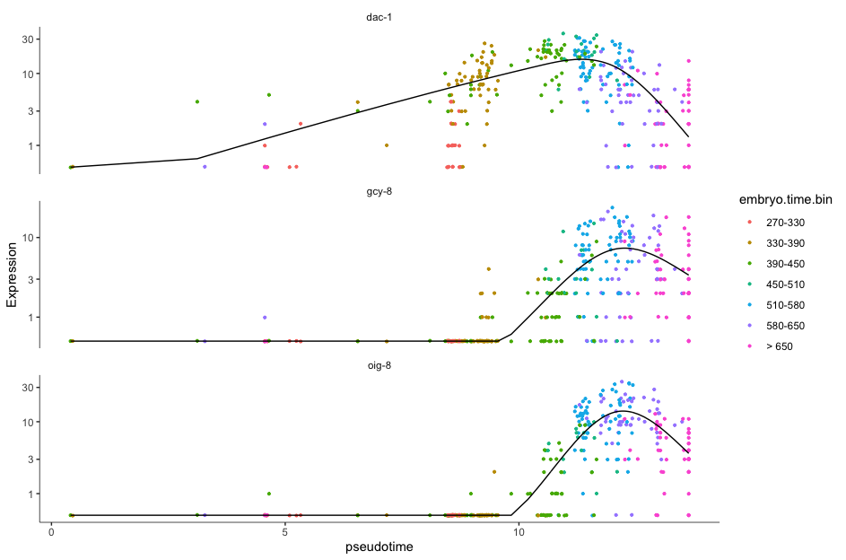
- We will choose AFD neuronal cells which are the main thermosensors in C.elegens.
- gcy-8 (Guanylyl Cyclase-8), dac-1 (Dachshund Homolog-1) and oig-8 (Immunoglobulin Superfamily Protein OIG-8) are the genes involved in thermosensation, neuronal development and neuronal connectivity.
**Step-1: Define the Genes of Interest**
AFD_genes <- c("gcy-8", "dac-1", "oig-8")
**Step-2: Subset the CellDataSet for AFD Lineage**
AFD_lineage_cds <- cds6[rowData(cds6)$gene_short_name %in% AFD_genes,
                        colData(cds6)$cell.type %in% c("AFD")]
- Subsetting rows:
rowData(cds6)$gene_short_name %in% AFD_genesfilters the dataset to include only the genes"gcy-8","dac-1", and"oig-8".
- The information about the pseudotime is stored within
AFD_lineage_cds@colData.
**Step 3: Plot Gene Expression Over Pseudotime**
plot_genes_in_pseudotime(AFD_lineage_cds,
                         color_cells_by="embryo.time.bin",
                         min_expr=0.5)
color_cells_by="embryo.time.bin": Colors the cells based on embryonic time bins, helping visualize gene expression patterns over developmental stages.
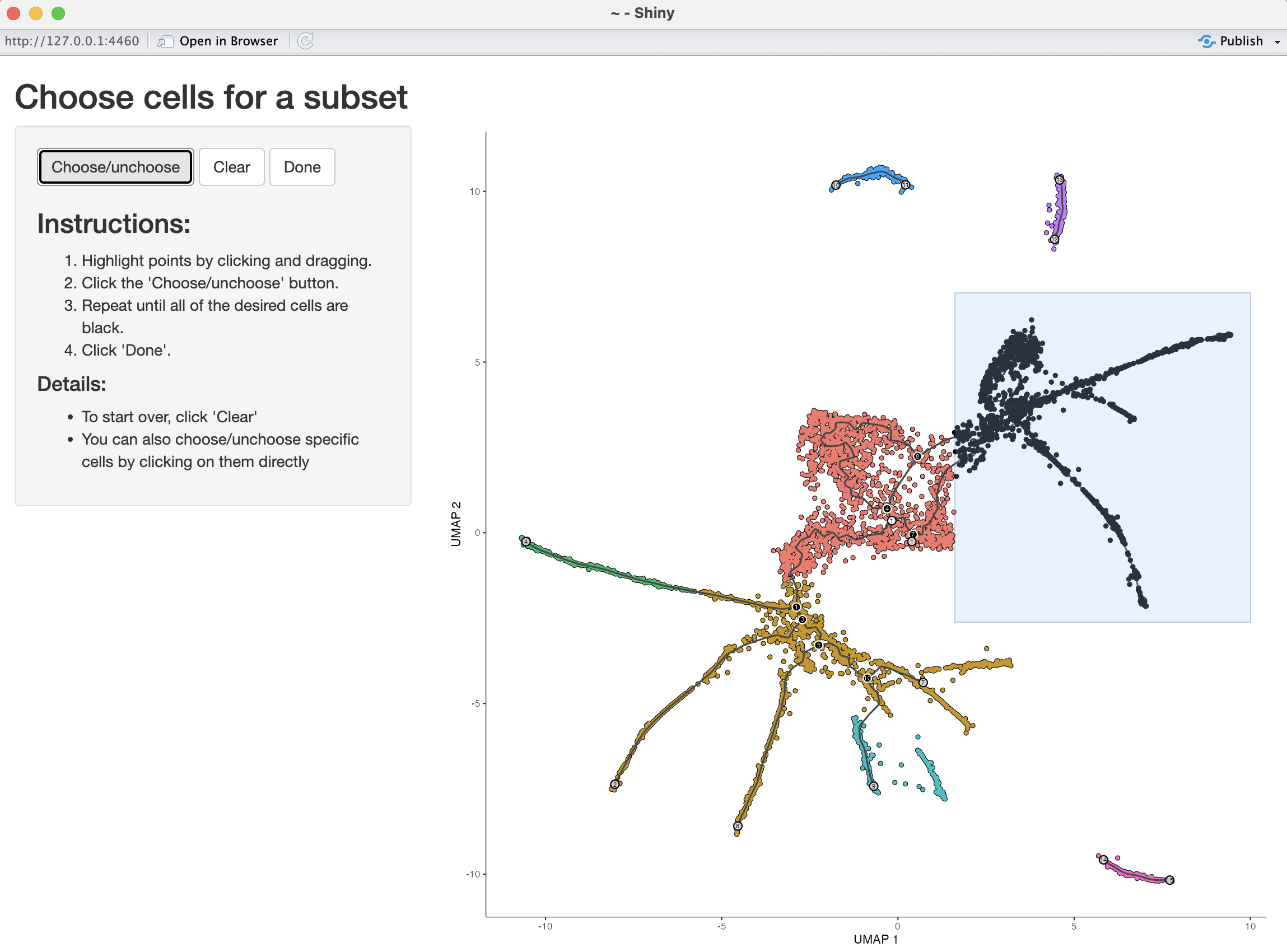
Analyzing branches in single-cell trajectories
- Analyzing the genes that are regulated around trajectory branch points often provides insights into the genetic circuits that control cell fate decisions.
- Monocle can help you drill into a branch point that corresponds to a fate decision in your system.
- You can do so by selecting the cells (and branch point) of interest using the
choose_cells()command:
cds_subset <- choose_cells(cds6)
- Use the
graph_test()on the subset. - This will identify genes with interesting patterns of expression that fall only within the region of the trajectory you selected, giving you a more refined and relevant set of genes.
- It identifies differentially expressed genes along the trajectory.
subset_pr_test_rescontains statistical results (e.g., q-values, p-values) for each gene.- The next command, filters genes where q_value < 0.05 (statistically significant).
- The gene IDs are stored in
pr_deg_ids
subset_pr_test_res <- graph_test(cds_subset, neighbor_graph="principal_graph", cores=4)
pr_deg_ids <- row.names(subset(subset_pr_test_res, q_value < 0.05))
- The next step is to find gene modules.
- The
find_gene_modules()function is used to identify groups of genes that show similar expression patterns across cells. - These groups, or gene modules, can help in understanding co-regulated genes, biological pathways, and cell-state transitions.
gene_module_df <- find_gene_modules(cds_subset[pr_deg_ids,], resolution=0.001)
- The next command
aggregate_gene_expression()is used to summarize gene expression levels across groups of cells based on gene modules or other annotations. - This helps in identifying patterns of gene expression across different cell clusters, pseudotime states, or biological conditions.
agg_mat <- aggregate_gene_expression(cds_subset, gene_module_df)
- The next step is to perform Hierarchical Clustering of Gene Modules.
- The command performs hierarchical clustering on the aggregated gene expression matrix.
module_dendro <- hclust(dist(agg_mat))
- In the next step, we need to reorder Gene Modules for Better Visualization based on hierarchical clustering results (
module_dendro$order).
gene_module_df$module <- factor(gene_module_df$module,
                                levels = row.names(agg_mat)[module_dendro$order])
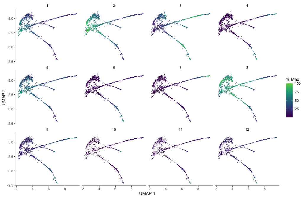
Finally we can visualize the Cells and Their Gene Expression which highlights expression of genes within each module.
plot_cells(cds_subset,
           genes=gene_module_df,
           label_cell_groups=FALSE,
           show_trajectory_graph=FALSE)